Introduction
Network theory has grown at a rapid rate in the last couple of decades. Researchers in a variety of disciplines are finding network concepts and measures to be useful tools for understanding and intervening in group structures organized around many types of interactions. Some of these include, for example, disease transmission (Morris & Kretzschmar, 1997; Sattenspiel & Simon, 1988), the internet (Albert et al., 1999), networks and communities of tweets (Peiper et al., 2017), the co-ownership networks of companies (Kogut & Walker, 1999), collaboration within a network of scientists (Newman, 2001a, 2001b), and protein interactions (Stumpf & Wiuf, 2005).
A major limitation of empirical network studies is that information regarding all of the nodes and connections in a network is rarely available. Whether because the boundaries of the complete network are unknown or because of incomplete or missing data (Morris, 2004; Stork & Richards, 1992), most network studies, especially in social studies, are typically based on a sample of the network. This also becomes important in the era of “Big Data,” when researchers use samples of rapidly generated data (e.g., Twitter) to proxy for full data sets.
Unlike social networks, airline networks can offer more measurable, reliable, and stable information about network structure, connections, and dynamics, which in turn can serve well for network sampling design study purposes. Further, airline networks contain clustering tendencies in the form of homophily effects—that is, similar airlines are linked together, as commonly seen in empirical/social networks. A collection of papers using airline transportation networks to describe the global spread of influenza illustrates the need for research on optimal sampling strategies. In particular, Rvachev and Longini (1985) use a strategically selected network of the 52 largest airports in the world to study the global spread of influenza. Grais, Hugh Ellis, and Glass (2003), Cooper, Pitman, Edmunds, and Gay (2006), and Epstein et al. (2007) respectively base inference solely on the 100, 120, and 155 largest airports, whereas Colizza, Barrat, Barthélemy, and Vespignani (2006) use the entire list of all 3,172 available airports. Complete population assessment for network studies is motivated by a concern that network measures become increasingly unreliable as sample fractions decrease (Burt, 1983). Stumpf, Wiuf, and May (2005) show that a random sample of nodes selected from a scale-free network are not themselves scale free, and Bobashev, Morris, and Goedecke (2008) provide the analysis of airport selection strategies to optimize the selection of airports for optimal performance of a global epidemic model.
The structure of a network depends on both its nodes and edges. Consequently, sampling from a network draws from two distinct populations: the set of nodes and the set of edges. A major challenge is to design a sampling method that produces representative samples of both nodes and edges. Because the two populations may often have some interdependence, care must be taken to avoid bias. For instance, in a heterogeneous network with proportionate mixing, one can show that randomly chosen neighbors of individuals (i.e., nodes found by following edges chosen at random) have a tendency to have more neighbors than do randomly chosen individuals (Newman, 2003). Notably, respondent-driven sampling attempts to consider both dimensions of networks by sampling from edges but then weighting the sample post-hoc to adjust for the tendency to oversample nodes with more edges (Heckathorn, 2002).
An understanding of the direction and magnitude of bias that different sampling techniques create in the estimation of network metrics would allow for more informed choices of appropriate network sampling techniques and better post-hoc adjustment of network calculations to approximate the true underlying network structure. The completion and size of airline networks provides a good exploratory test bed for network theories. In this paper, we use an empirical network created by worldwide flight connections between airports to explore the impact of different sampling designs and sampling fractions on the characteristics of the sample. We compare measures of network structure and volume of transportation (i.e., the total number of seats available for travel) in the sample networks with the same measures based on the complete network. We show the extent of the similarity between sampled networks and the completely enumerated network, considering both the nodes and edges of the networks. In addition, we seek to understand the dependencies, if any, of the network measures on the sampling designs and sample sizes.
Terminology
Network analysis, as with most scientific disciplines and distinct analytic approaches, carries its own set of terminology. In this manuscript, we refer hereafter to the airports in this network as the “nodes” and the connections between them as “edges.” Specifically, an edge exists between two airports if there are scheduled flights between them over a fixed period of time. Edges between nodes can be binary (0,1) or “unweighted” if the flight volume is ignored, or “weighted” if flight volume is acknowledged; the weighted edges will then have a range of values corresponding to the transport volume. We selected and calculated several network measures that are common in social network analysis and that we considered to be potentially useful for the characterization of transportation networks. These measures include degree, geodesic length, transitivity, and centralization and are further defined in the methods section.
Data
We use flight information reported by commercial airlines to the OAG (formerly the Official Airline Guide) during calendar year 2004. The OAG estimates that 99 percent of all commercial airlines report their daily scheduled flight information to the OAG at different intervals throughout the year (https://www.oag.com/). For each scheduled flight, the airlines report the number of seats on that plane and the three-character airport codes corresponding to the cities of origin and destination. Airport codes typically corresponded to distinct cities. However, for some of the larger metropolitan areas the OAG aggregates airports at the city level. For example, the NYC (New York City) code includes JFK (John F. Kennedy), LGA (LaGuardia), and EWR (Newark) airports. The OAG flight schedule for 2004 contains information about flights between 3,687 cities. Specifically, we aggregated 214 airports in 96 cities and removed 8 airports from this analysis because they were connected only to each other and not to any other airports. After removing these 8 nodes, 3,679 nodes remain for the analysis. If airports are connected by scheduled flights, then we consider them as being connected. For a small number of airports, the connection is unidirectional. Because the percentage of these flights is small—less than 0.6 percent of all flights—for the purposes of our theoretical analysis, we consider the corresponding airports as connected. Some characteristics of these transportation networks are discussed in Bobashev et al. (2008). All network plots are made in R with “igraph” package (Csardi & Nepusz, 2006).
Methods
We apply three sampling designs to the airport network: (1) simple random sampling (SRS), (2) strategic sampling of the largest cities (SSLC), and (3) controlled snowball sampling (CSS). CSS can be considered an ideal implementation of respondent-driven sampling for this study. The designs are chosen to reflect a variety of empirical assumptions and approaches to sampling from networks.
SRS requires the entire sample frame to be known. Each node has an equal probability of being selected for the sample. For example, if the sample size is 100 and the population size is 1,000, then each population unit will have a probability equal to 10 percent of being selected for the sample.
In some cases, one may want to base the selection probability on the “importance” of the airport. For example, one might want to ensure that some large airports are selected for the sample by assigning larger probabilities of selection to such airports. An extreme case of such an approach would be when the largest airports are selected with certainty and the smallest are selected with probability zero. We explore such an extreme case and refer to it as “strategic sampling” (also known as “cut-off sampling”). A strategic sampling design can result in a loss of representativeness of the entire network because smaller airports will not be sampled. However, an advantage to using such a design is that it will capture and reflect the majority of the transportation flux.
CSS starts with a set of randomly selected nodes and then proceeds using a chain referral sampling design such that at each wave a set of edges/links from each selected node are selected to be traced for the sample. Figure 1 presents an example of a sample selected via a variant of a CSS design applied to a simulated population.
CSS is especially useful when the entire population is not known because it allows one to obtain a sample of conspicuous units fairly quickly by “digging” deep into the network; nodes with large-degree are more likely to be sampled than nodes with small-degree. For example, starting with any randomly selected airport a sample will soon reach the main hubs and follow the main traffic routes; see Figure 1. Because CSS is based on selecting network links to trace, and not nodes, unconventional analyses are required to obtain efficient estimates.
We set sample sizes to five proportions of the population size, 3,679, namely 75, 50, 25, 10, and 3 percent of this value. These choices are based on practical reasons. For example, we choose 3 percent of the total number of cities to obtain a sample size approximately equal to 100. Large sampling fractions correspond to network surveys when a small fraction is not reachable or responding.
Because the strategic samples are unique, they are selected only once. For the other sampling designs, we select 50 samples at each sampling fraction and then calculate the mean of the sample characteristics over the set of samples. We also calculate standard deviations of the distributions of the estimates, and present these as error bars in Figures 6 through 13 in the Results section.
Sample Selection
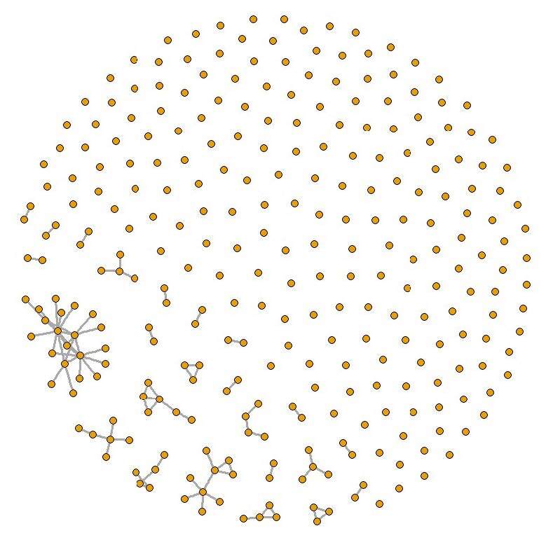
We assume that all connections between cities are known, and once cities are selected for the sample, we include observations of the direct flight connections between all pairs of sampled nodes/cities. Figure 2 presents a simplified visual illustration of the complete network graph. Because most of the airports are connected to a small number of airports, the actual complete network would resemble a “cloud.” In Figure 2, we depict a “backbone” of the network, representing highly connected nodes.
For the SRS design, a sample of nodes is selected completely at random from the set of nodes in the complete network. Figure 3 illustrates an SRS equal to 10 percent of the population size when sampled from the complete network.
For the strategic sampling design, we first rank the cities based on their volume of air traffic (as measured by the total number of seats) and then select cities in order up to our target sample size; sampling in this manner is equivalent to selecting the tail of the degree distribution. Figure 4 illustrates a strategic sample equal to 10 percent of the population size when sampled from the full network.
Controlled snowball sampling is a link tracing–based strategy in which cities are selected for the sample as follows. First, seven cities are randomly selected for the “seed” portion of the sample. Then, between zero and seven additional cities to which each sampled city has flight connections are selected, and so on, until the desired sample size is obtained. The number of links to trace is chosen from a binomial distribution with parameters n = 7 and P = 5/7. Such selection is typical for respondent-driven samples because it removes strong clustering effects that can occur in a snowball sample without such restriction. A smaller number of selected links leads to smaller dependence of the selected sample from the initial seed. If a city is selected that has already been included in the sample, then it is not allowed to include additional flight connections but does count toward the total number of selections for its recruiter. For instance, if Atlanta, Miami, and Charlotte are traced from Raleigh-Durham, and then Los Angeles, Denver, and Raleigh-Durham are traced from Atlanta, we include Raleigh-Durham as a link traced from Atlanta’s network, but we do not allow any more cities to be traced from Raleigh-Durham. Up to seven links are traced because this number has been successfully used in practice in the social network area and provides a good balance between being able to obtain representativeness of the graph while achieving target sample sizes. Figure 5 illustrates a CSS with a target size of 10 percent of the population when sampled from the full network.
With the CSS design, links from sampled cities are allowed only one opportunity to be traced to select additional cities into the sample. Sampling ceases once all cities in the sample have had this opportunity. This “saturation point” may occur before the sample size reaches its target level, especially when the targeted sample size is large. To overcome this limitation, more convenience seeds could be selected. A primary feature of respondent-driven sampling (which is essentially what CSS is) is that it leads to a representative sample when long recruitment chains are obtained, regardless of whether the seeds were selected at random or conveniently (Heckathorn, 2002). This allows one to select convenience seeds, possibly within each country of high interest to the researcher.
Measures
For each sample, we evaluate five metrics that network studies commonly use: average symmetrized node degree, network centralization, average geodesic length, network density, and network transitivity. We also determine the percentage of isolated nodes and total air traffic accounted for by the sample.
Degree
Degree is the term used to refer to the number of edges emanating from (out-degree) or returning to (in-degree) a node. Because the data are symmetrized, we determine the symmetrized degree measure. Typically, degree is used as a measure of node centrality in the network. However, we are interested in the distribution of degree in the network. We calculate the average symmetrized node degree as the mean of the symmetrized node degree across all sampled nodes. This measure can be useful to compare two or more networks with relation to the average number of connections per node. A second characteristic of interest is the variance of the degree distribution, which characterizes heterogeneity in degrees among the nodes.
Network Centralization
Network centralization describes how well-connected nodes are in a network in relation to the size of the network. Network centralization scores can range from 0 (completely decentralized) to 1 (completely centralized). A centralized network is dominated by one or a few very central nodes. A network with a centralization score of 1 would look like a star with all nodes connected through one central node or “hub” (hubs are nodes with high degree and centrality). Note that if the hubs are removed from a network, it fragments into unconnected subnetworks. A network with a centralization score of 0 would be a network with no links present.
We calculate network centralization, denoted by CD, using Freeman’s (1978–1979) formula as
CD=g∑i=1[CD(n∗)−CD(ni)](g−1)(g−2)
where CD(ni) is the degree of node i, CD(n*) is the maximum of CD(ni) across all i, and g is the number of nodes. The denominator corresponds to the maximum possible centrality (when the nodes are arranged as a star) and is used to ensure the scores fall between zero and one. Network centralization is zero when all nodes have the same centrality.
Network centralization is important for airline transportation because it characterizes how much the network “depends” on the hubs. Such characteristics might not be of high interest when all airlines are considered but is crucial for comparing routing structures between different airlines.
Geodesic Length
The network term “geodesic” is used to refer to the shortest path between any two nodes in a network. The average geodesic length gives a sense of how many steps it takes on average to travel between any two points in the network. This characteristic is critical for transportation research, especially for airline transportation, because it reflects availability of direct flights and the number of flight changes en route from one city to another.
Network Density
Network density is the proportion of edges in a population network relative to the total number of possible edges in the population network. This measure can be used to classify networks as either “sparse” or “dense.” A network is considered dense if a large fraction of edges exist. If the fraction of edges is small, then the network is said to be sparse. This measure is somewhat related to geodesic length because it characterizes the amount of connectivity between nodes. However, unlike geodesic length, density is a simpler and cruder measure.
Network Transitivity
Broadly speaking, network transitivity measures how often pairs of connected nodes share common neighbors. Sometimes, network transitivity is called “cliquishness” of the network. A pair of connected nodes sharing a common neighbor leads to the appearance of a triangle in the network. However, if one node in the pair has a neighbor that is not shared with the other node in the pair then this leads to a path of length two that does not close into a triangle. The network transitivity is calculated as
C = 3 × (number of triangles) / (number of paths of length two). (2)
The denominator includes paths of length two that close into a triangle and those that do not. Because a triangle gives rise to three paths of length two but just one triangle, the numerator includes a factor of three. This ensures that C = 1 when all paths of length two close into a triangle. This definition is different from the one that Watts and Strogatz (1998) use, which considers all edges attached to a node instead of focusing exclusively on triangles. For transportation purposes, transitivity can indicate connections between cities through direct and single connection flights.
Percentage of Isolated Nodes
The percentage of isolated nodes may not be considered an important measure for connected transportation networks, but it has utility in illustrating how sampling designs can select cities that are not connected to other cities in the sample. The measure grows in importance when sampling effort is directed toward smaller cities. To determine the percentage of isolated nodes in a sample, we divide the number of nodes having no edges (nodes of degree 0) by the total number of nodes in the network.
Percentage of Total Air Traffic
The percentage of total air traffic represented in a sample is determined by dividing the volume of air traffic captured by the sample by the total volume of air traffic in the completely enumerated network. The volume of air traffic is measured in available seats.
All network measures, calculations, and data management are performed using R software.
Results
Characteristics of the Complete Network
The completely enumerated network created by flight connections between cities has several distinctive features. For one, the completely enumerated network that we use as our reference network is symmetric. In addition, there are no isolated nodes in the network. The completely enumerated network also has characteristics of a scale-free network (Barabási & Albert, 1999) in that many cities have just a few connections and a few cities are network hubs (i.e., are connected to a large number of other cities). This property is demonstrated in Figure 6, which shows the highly skewed degree distribution.
The 100 most connected cities, which make up 2.7 percent of all cities, are end points on 30.6 percent of all connections in the completely enumerated network. Colizza, Barrat, Barthélemy, and Vespignani (2006) found that the degree distribution for most airports, with the exception of the most connected airports, follows a power law distribution. Such heterogeneity in degree distribution is likely to have a strong impact on sample features and should therefore be considered when interpreting the results of the study.
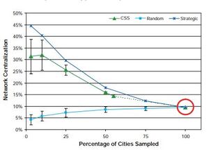
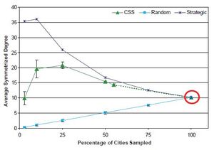
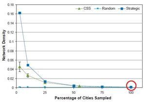
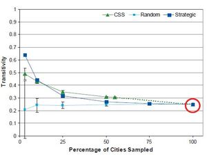
In the following subsections, figures are used to summarize the findings. We highlight the value of each measure based on the completely enumerated network, via a circle drawn around it, because this is taken to be the relevant point of comparison for all other numbers in the graphs. We also plot the CSS-based measures such that measures based on samples with a 75 percent target sampling rate are actually plotted at 55 percent (the average of the realized sampling rates for these samples). As discussed previously, the CSS sampling strategy does not always achieve the target sampling rate, so we plot the realized rate instead of the target rate. In addition, we connect the 55 percent point to the 100 percent point with a dotted line. This indicates that although it is theoretically possible to generate samples with sampling rates in this range, such samples are unlikely to be selected when sampling from the air traffic network. All 50 CSS samples we generate with a target sampling rate of 75 percent reach their saturation point before they reach the target size. The realized sampling rates range from a minimum of 50.2 percent to a maximum of 59.0 percent, with a mean of 55.1 percent and a median of 54.9 percent. Of the CSS samples with target rates of 3, 10, 25, and 50 percent, only one fails to reach its target sampling rate. In this particular sample, the target rate is 50 percent, but the realized rate is 49.7 percent.
Network Centralization
As Figure 7 shows, the completely enumerated network is not highly centralized; the network centralization equals 0.1. In this figure, the random sample shows the opposite trend of the strategic and CSS sampling methods. Although network centralization decreases with the SRS design over decreasing sample sizes, it increases with the strategic and CSS designs.
Average Symmetrized Degree
In Figure 8, the measured average degree is displayed across the sample sizes. With the SRS design, the average node degree drops to close to zero (0.29) connections at the 3 percent sampling level. The interpretation of an average degree of zero is that there are no connections between the remaining nodes. With the strategic sampling design, the average degree increases as the sampling fraction decreases. The CSS design gives rise to results that are similar to those found with the strategic sampling design because the most connected cities are more likely to be selected for the sample. At the lowest sampling fractions (i.e., 10 and 3 percent), however, the CSS sample falls back to the average degree most similar to that in the completely enumerated network.
The results based on the strategic and CSS sampling designs approach the average degree, which reflects the effect of network hubs whose presence was demonstrated in Figure 7. Because the strategic sampling design operates with respect to volume of air traffic, the sample typically includes cities with the highest degree (i.e., the hub cities) and therefore overestimates the average degree. In contrast, with the SRS design, hub cities are no more likely to be selected than any other city. With the CSS design, as the sampling fraction increases, we first see an increase in average degree and then a decrease. One possible explanation for this behavior is related to how rapidly the hubs are selected for the sample. Unlike the strategic sampling design, in which the largest hubs are likely to be selected first, the CSS design chooses the initial set of cities randomly. Hubs are typically added to the sample only via their connections to this initial sample (and then subsequent) waves of sampling. Once hubs are reached, the average degree should start to increase. Then, as the sample size continues to increase, a point is eventually reached at which the hubs are exhausted and less well-connected cities start making up a larger portion of the sample, thus decreasing the average degree.
Average Geodesic Length
In Figure 9, we present the distribution of the average length of geodesic paths in the largest connected component for samples selected under each design; because sampling typically results in a set of disconnected network components, we report the average geodesic length solely for the largest connected component. We choose to examine the path lengths in this component because path lengths connecting smaller components are shorter, on which estimates may be further biased. Starting at a sampling fraction equal to 100 percent, the average geodesic length reported with the SRS design stays at approximately the same length as in the complete network until less than 50 percent of the population is selected. In comparison, the strategic sampling design results in a continual decline in average geodesic length across decreasing sampling fractions. The length of the average geodesic reported with the strategic sampling design is monotonic because even with the smallest sampling fractions almost all sampled cities are likely to be connected with each other (i.e., with a geodesic of 1).
Network Density
As Figure 10 shows, the completely enumerated network is very sparsely connected because only a small proportion of total possible flight connections exist (density = 0.001). SRS is best for preserving this characteristic across decreasing sampling fractions, whereas density is overestimated by both the strategic and CSS sampling designs. At the smallest sampling fractions, the strategic sampling design selects nodes that are highly connected to each other and therefore substantially overestimates the network density.
Network Transitivity
As Figure 11 shows, for each sampling design, when at least 50 percent of the population is sampled the estimated network transitivity coefficient stays within 10 percent of the original measure. At sampling fractions less than 50 percent, the SRS design results in a different trend than that given by the strategic and CSS designs. Although the transitivity coefficient with the SRS design stays nearly the same or decreases slightly as the sampling fraction decreases, with the strategic and CSS designs it increases.
Percentage of Isolated Nodes
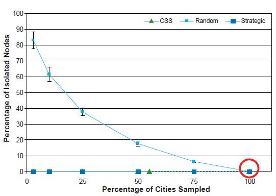
As previously noted, there are no isolated nodes in the completely enumerated network. As the sampling fraction decreases, the percentage of isolated nodes increases substantially with the SRS design, in contrast to the SSLC and CSS designs, in which there is almost no change in the percentage of isolated nodes; see Figure 12. The percentage of isolated nodes with the CSS design is always zero, and for the strategic sampling designs, it is either zero or very near zero. The CSS design, by virtue of selecting new nodes based on their connections (edges) to other nodes, is guaranteed to give no isolated nodes. The large percentage of isolated nodes typically selected with the SRS design reflects the sparseness of edges in the original network.
Percentage of Total Air Traffic
Finally, we examine the percentage of total air traffic accounted for by the sample. Total air traffic refers to the total number of edges that come from the sampled nodes, and we count each seat as a separate edge to better approximate the number of agents traveling in this network. In Figure 13, we observe that the percentage of total air traffic is best reflected with the strategic sampling design and least with the SRS design.
Conclusions and Discussion
By using data from a completely enumerated network, we are able to show how different types of sampling designs and sample sizes influence network metrics calculated from the resulting samples. Overall, an SRS design shows the best performance in preserving the centralization, density, and transitivity metrics. However, unlike the CSS design, it requires knowledge of the entire population. When large airports are oversampled either through strategic or CSS design, many of the network features become significantly biased. This is especially evident with small sample sizes. These findings have implications for researchers in a variety of disciplines because they highlight the necessity of giving sufficient consideration to the choice of sampling design.
The findings presented in this paper indicate the potential to infer on characteristics of the complete network post hoc if the sampling design and size are known or can be reasonably approximated/inferred. For example, if one uses an SRS design and has an idea of what the sample size may be, then one can consider a set of subsamples and extrapolate the network characteristic curves to estimate what they could be for the entire population. This technique would allow one to simulate networks with such known characteristics, which could then be used in future studies.
The results presented in this paper should follow the intuition behind network and sampling design studies. CSS, by virtue of selecting nodes that are connected to the existing sample, will never produce an average degree of zero. SRS should result in some nodes typically being unreachable because, as mentioned, most cities in the sample have a small number of other cities to which they are directly connected. As a result, as the sample size decreases, the chances of selecting one of these direct connections also decreases. Finally, cities selected via the strategic sampling design are typically connected across decreasing sampling fractions and continue to account for a large proportion of air traffic. Such findings result from the design as it is developed to best account for air traffic.
Heterogeneity of the degree distribution drives the results found in this study. For example, SRS results in the selection of some weakly connected nodes and so explains why, for small sample sizes, the samples result in a low average degree. As the sample size is increased, a more connected graph is bound to be observed. If the degree distribution in the underlying population were more homogenous, then the connectivity of the graph would not differ so substantially at different sampling levels. Similarly, the CSS design is affected by degree heterogeneity. Because seeds are chosen at random at the start of sample selection, the connected nodes (neighbors) selected for further observation should be responsible for the increase in the sample average degree. If neighbors have a higher connectivity than the population average degree, then the sample degree will increase with the sample size. An extreme example of this can be illustrated with a star-structured graph, in which a peripheral node is most likely to be selected for the initial sample. This node has only one connection to the central node, which has many more connections but is less likely to be selected for the start of sampling (Feld, 1991). CSS sampling will sample only less-connected nodes once highly connected nodes are already included in the sample.
The findings presented in this paper have important implications for those planning to collect or analyze real-world network data and mathematical modelers who are interested in modeling network processes. For instance, our findings indicate that the SRS design maintains a low level of centralization, whereas the CSS and strategic sampling designs overestimate the level of centralization. Therefore, if one aims to model a network using a sample of network data, perhaps to study the diffusion of disease or goods throughout the network, a strategic or CSS sample is likely to predict more rapid diffusion than an SRS by virtue of giving too much credit to a few highly centralized nodes. However, if one relies on an SRS to estimate the average number of pathways (edge degree) across which an agent can travel between nodes, then they are likely to underestimate this metric because the sample will not necessarily include the hub airports. For the same reason (i.e., not including hub airports), if the question of interest is efficiency of spread in a network, then the sample is likely to provide a better estimate of the geodesic lengths in the network than a strategic or CSS sample, which is likely to underestimate geodesic lengths by virtue of including highly connected airports. Finally, if the question of interest has more to do with accurately estimating the quantity or volume of edges in the network, the strategic sample in which hubs are included is best equipped to answer this question.
Each sampling strategy brings a different perspective on uncertainty. For example, with SRS, as one could expect, the variability of estimated characteristics decreases as the sample size grows larger. Strategic sampling doesn’t have any variability or randomness because it is a non-random selection of the top cities. With CSS the uncertainty decreases quickly because the sample quickly reaches most connected nodes. This issue is related to another important research topic of generating representative samples (e.g., bootstrap samples) from a network. For bootstrap the variability is critical, but at the same time there is a need to reproduce distributions of certain network characteristics such as centrality Gel et al. (2017). At the same time, bootstrap techniques that preserve centrality might not be the best ones to represent clustering. Simulation studies like ours highlights the importance of understanding how the data was collected.
In many studies, the choice of sampling design is governed by information about the network, available resources, privacy considerations, and so forth. The results presented in this paper encourage researchers to consider the effects sampling design can have on the resulting sample network structure.
Several caveats accompany these findings. For one, although we are considering the OAG data that we used to be a completely enumerated network, there is likely a small amount of missing data in this network as there are other smaller airports and airports used by private airlines that do not show up in the OAG data. Also, this study is limited to exploring three sampling designs. There are several other ways in which networks can be sampled (e.g., uncontrolled snowball sampling, contact-tracing, random walks). Perhaps most importantly, when attempting to generalize from these findings what one might expect in other networks, it should be kept in mind that the results presented here are also likely to be dependent on the structure of the network we choose to analyze.
Note that, when sampling, we assume all connections are known and thus we are reconstructing the true underlying structure of the network. In real-world social and transportation networks, the true underlying structure of a network is often unknown. For example, ground transportation patterns dynamically change, especially in developing countries. When connections are known with uncertainty, probabilistic methods are sometimes used for the reconstruction of the connections. In our study, we have not addressed the additional level of uncertainty that is introduced by inexact knowledge of the connection.
Acknowledgments
This work was supported in part by the Pilot Studies of Modeling of Infectious Disease Agents Study (MIDAS), grant number 1 U01 GM070698, and the SATH-CAP project, grant number UO1 DA017394.


