Addressing Nonresponse for Categorical Data Items Using Full Information Maximum Likelihood With Latent GOLD 5.0

Introduction

Nonresponse can occur for several reasons including refusals, inconsistent or invalid responses, “don’t knows,” and inadvertent skips. In the statistical literature, nonresponse is assumed to arise from three types of stochastic mechanisms (see, for example, Rubin, 1976). Missing completely at random (MCAR) occurs when the nonresponse is completely unrelated to independent or dependent variables (i.e., not dependent on any attributes); missing at random (MAR) occurs when the nonresponse is related to the observed information but not the dependent variable(s); and missing not at random (MNAR) occurs when the nonresponse is not MCAR or MAR.

Regardless of the underlying mechanism, ignoring missing data in a data analysis can lead to biased and/or inefficient inference. Fortunately, many techniques have been developed to handle missing data. Some common techniques are listwise deletion and single imputation including mean imputation, hot deck imputation, and predictive mean matching. Multiple imputation and full information maximum likelihood (FIML) are among the newer techniques that can yield unbiased inferences and valid standard error estimates. Asymptotically, multiple imputation can yield results that are identical to those obtained using FIML (Graham, 2009; Little & Rubin, 2002).

Several statistical software packages have incorporated methods for addressing nonresponse. Some of these are LEM, MPlus, SAS, Stata, R, and Latent GOLD (LG). Implementing more standard approaches for handling missing data is quite often straightforward in these software packages; for instance, regression analyses using SAS and Stata employ listwise deletion by default. However, implementing more complex missing data techniques may require a more intimate knowledge of the software and the data.

This report provides a primer for applying FIML to compensate for missing data in log-linear models for users of LG. While not detailed in this report, the techniques presented can apply to latent class models (see the supplementary article materials published with Edwards, Berzofsky, & Biemer, 2017 for LG code applying these techniques to Markov latent class models).

Two methods for handling missing data in LG are well documented and specified as user options: complete case analysis (i.e., listwise deletion) and FIML using Fuchs’ (1982) method, which assumes MAR (Vermunt & Magidson, 2005, 2016). The latter method can only be applied for missing data in the dependent variables and automatically invokes mean imputation to address any missing data in the independent variables. Although Fuchs’ approach works well for MAR data, the method by Fay (1986) is more general; it can be applied for both MAR and MNAR nonresponse by incorporating and modeling item nonresponse indicators. Unfortunately, Fay’s method is not a user option in LG; however, it is not difficult to set up the LG software to force-fit Fay’s method for handling missing data, as we show for MAR nonresponse in the section Modeling Assuming Data Missing at Random (MAR). The section Modeling Assuming Data Missing Not at Random (MNAR) describes in detail how to model item missing data for all variables in categorical data analysis using LG models when the missing data mechanism is MNAR. Doing so allows us to model both MAR and MNAR missingness for both dependent and independent variables. This makes LG unique since Fay’s method is not available in any other data analysis software packages to our knowledge.

The rest of this introduction discusses missing data mechanisms, FIML assumptions, and available software packages in more depth. The Methods and Results section details the LG syntax for fitting FIML models using two different approaches (Fuchs’ and Fay’s) under each response mechanism for both dependent and independent variables. The discussion summarizes these various methods and discusses potential difficulties with implementing each approach.

Missing Data Mechanisms

Every imputation method makes assumptions about the causal nature of the missing data; this is known as the missing data mechanism. Nonresponse is often classified according to one of three missing data mechanisms: missing completely at random (MCAR), missing at random (MAR), or missing not at random (MNAR). Originally defined by Rubin (1976), MCAR occurs when the missingness does not depend on either the observed or unobserved data; MAR is a less restrictive assumption in that the missingness depends only on the observed data; and MNAR is the least restrictive mechanism regarding modeling assumptions, where the missingness depends on both the observed and unobserved data.

Under MAR and MNAR the respondents and nonrespondents may differ on the outcome variable of interest. Under a MAR mechanism, the missing outcomes are explained by other observed independent variables, so the response mechanism is assumed to be ignorable conditional on these observed independent variables. Under a MNAR approach, the missing data mechanism interacts with the outcome variable. This interaction can be expressed using a response indicator to incorporate information regarding the response mechanism into the imputation model (Rubin, 1976). Thus, to model MNAR data, the observed data and the response mechanism must be modeled jointly to account for observed and unobserved influences on the missingness.

Current approaches to modeling MNAR data can be classified into two types: selection models and pattern mixture models (Heckman, 1976; Little, 1993). Selection models require fitting a two-part model—with one model for the outcome variable and another model for the response mechanism given the outcome variable. Pattern mixture models form subgroups of cases that share the same missing data pattern and then fit a model for each pattern. The overall model is then estimated using a weighted average of the individual models; standard error estimates for a pattern mixture model are often estimated using the delta method (Enders, 2010). Formulas for these models are presented in Table 1, where Y is the incomplete outcome variable of interest and R is a response indicator of Y.

These MNAR techniques require strong assumptions about the data in order for the models to be identifiable (that is, to contain reliable estimates). Selection models assume that the underlying response probabilities and the incomplete outcome variable follow a bivariate normal distribution. Pattern mixture models require the researcher to specify values for the inestimable parameters and have largely been used in conducting sensitivity analyses (Enders, 2010). When these assumptions are met, and the missing data mechanism is MNAR, simulation studies have shown that these methods tend to inflate the variance estimates (Fay, 1986). Our report addresses MNAR missing data through a selection model approach. For more information on pattern mixture modeling, refer to Little (1993) and references citing Little (1993).

Full Information Maximum Likelihood (FIML)

When the general conditions for estimation are satisfied, FIML methods can be used to fit a structural (or substantive) model for the outcome variable and nonresponse model simultaneously. While not an imputation method, FIML makes use of all available data (including partially observed data) to maximize the log-likelihood of this joint model (Enders, 2010). A considerable amount of work has been done around applying FIML under a MAR response mechanism and modeling MNAR data with a continuous outcome (Anderson, 1957; Arbuckle, 1996; Graham, 2003; Little & Rubin, 2002).

For analysis of categorical dependent variables, FIML approaches are similar to those developed to handle continuous data in that partially observed information is used when maximizing a log-linear likelihood function. The primary difference is in the assumption about the sampling distribution: continuous data analysis assumes normality, and categorical data analysis assumes a multinomial sampling distribution (Vermunt, 1997).

If the data follow a MAR (or MCAR) response mechanism, this implies the response probabilities are independent of the missing variables. In this case, the likelihood can be factored into two components—one for the log-linear parameters and another for the response mechanism:

$\log\mathcal{L}_{(\pi,\Theta)} = \log\mathcal{L}_{(\pi)} + \log\mathcal{L}_{(\Theta)}$ (1)

where the structural probabilities are represented by $\pi$ and the response probabilities are represented by Θ. Under the MAR assumption, only the structural parameters need to be estimated since these two components can be maximized separately and the response mechanism is ignorable.

In 1982, Fuchs extended the methodology of FIML to estimate the parameters of a saturated log-linear model using the estimation-maximization algorithm when item nonresponse is ignorable. The chi-squared statistic of model fit resulting from the saturated MAR model jointly tests the MCAR assumption and the model fit. When the nonresponse mechanism is MNAR, this approach is not appropriate because, in that case, the log likelihood does not factor, as shown in equation (1).

Fay extended the FIML methodology to model the response mechanism by using recursive causal log-linear models which treat the response indicators as dependent variables, thus providing a FIML technique that applies to data with either nonignorable nonresponse (MNAR) and ignorable nonresponse (MAR or MCAR). In Fay’s approach, which uses a selection model, response indicators are created for all variables with partially observed data, and outcome and nonresponse models are fit using their joint likelihood.

Software Packages

Many programs are capable of applying FIML approaches to handle MAR missing data. A few of these programs include LEM, MPlus, SAS, Stata, R, and Latent GOLD (LG). While all of these packages are widely used, LG is specifically designed to analyze nominal, ordinal, and interval-level categorical data by assuming a multinomial sampling distribution with the capability to account for complex survey designs. LG fits all models as log-linear models, which can be conceptualized as mixture models. In LG, missing data are addressed by default through Fuchs’ FIML approach for dependent variables and a stochastic mean imputation for independent variables (Vermunt & Magidson, 2016). With some adjustments that are not documented in the 5.0 user manual, LG can accommodate both Fuchs’ and Fay’s FIML approaches on all variables with nonresponse in the log-linear model.

MPlus is a popular package used in structural equation modeling to analyze continuous, ordinal, nominal, and count data; MPlus can address a complex survey design and apply FIML to missing data. MPlus assumes a normal sampling distribution to implement FIML on categorical variables (Muthén & Muthén, 1998). Due to the distributional assumptions, these models are not fit as log-linear models. While this approach may be logical for binary, ordinal, or interval-level categorical variables, its effectiveness when used on nominal categorical variables is unclear. We are unaware whether MPlus can apply FIML in a log-linear model. Although MPlus handles MNAR missing mechanisms for continuous variables in a FIML construct, for categorical MNAR response, multiple imputation is the suggested approach (Asparouhov & Muthén, 2010).

This report focuses on using LG 5.0 to account for missing data, with particular focus on highlighting a technique to use Fuchs’ and Fay’s FIML approaches to address item nonresponse through the syntax module. These features of LG can make applying FIML to variables with MAR and MNAR nonresponse more accessible to researchers, as shown in the following section.

Methods and Results: Implementing the Full Information Maximum Likelihood (FIML) Technique

Modeling Assuming Data Missing Completely at Random (MCAR)

Fitting a model using cases where all data points are observed (i.e., listwise deletion or complete case analysis) is one of the easiest methods to implement to account for MCAR data. A path diagram of an MCAR model with four complete independent variables and one dependent variable with missing values is shown in Figure 1.

Figure 1.Missing completely at random (MCAR) model path diagram

In LG 5.0, complete case analysis is requested in the options section of the syntax code with the keyword “missing excludeall” (line 6 of Figure 2). In Figure 2, a main effects multinomial-logistic model for the dependent variable Y is defined with covariates A, B, C, and D using only observations with complete data for variables Y, A, B, C, and D. In Figure 2, all variables are multinomial. If Y is a binary variable, a log-linear logistic model is fit; if Y has more than two levels, a log-linear model is fit. In later figures we illustrate applications of FIML using binary variables for simplicity; these models can easily be extended to higher level multinomial variables, either ordinal or nominal.

Figure 2.Listwise (MCAR) model syntax in Latent GOLD 5.0

The LG syntax code consists of three sections—options, variables, and equations. The options section is used to set and turn off features available in LG. In the options section of LG 5.0, Bayes smoothers can be set to prevent boundary solutions, Monte-Carlo simulation requested, and power calculation methods invoked, although this is not shown in Figure 2. Refer to the LG technical manual for more guidance on how to implement these options. The variables section is used to declare all dependent, independent, and latent variables. Latent variables are unobserved variables that are inferred from other observed variables; they can be either continuous or categorical. Elements of a complex survey design would also be set in the variables section. Finally, the equations section contains any models of interest.

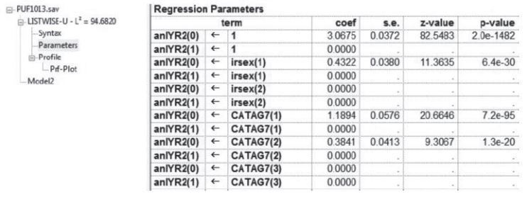
Once executed, LG creates several windows of output—Model Summary Output, Syntax, Parameters, and Profile. The Model Summary Output provides information on the model—the number of observations used to fit the model, the number of parameters in the model, seed values, and fit statistics—and can be viewed by clicking on the model name. Any warning or error messages regarding model estimation are listed in this window. The Parameters window contains model estimates for every model specified in the equations section of the syntax. Figures 3 and 4 contain example screenshots of the Model Summary Output and Parameters windows, respectively. For more information on the output windows refer to the LG users guide.

Figure 3.Example model summary output from Latent GOLD

Figure 4.Example parameters output from Latent GOLD

Modeling Assuming Data Missing at Random (MAR)

Models that implement a MAR mechanism can be fit a variety of ways using either a saturated MAR (Fuchs’) or response indicator (Fay’s) FIML approach. These methods are detailed in Table 2. Mean imputation is included as an option for the independent variables since it is the default method for handling item-nonresponse in independent variables in LG. From here on, we refer to models by model type, which is an abbreviation of the missing data approach applied to the dependent and independent variables, separated by a hyphen.

Figure 5.Missing at random (MAR) model path diagram

A path diagram showing the relationship between an outcome variable, its response indicator, and four independent variables in a MAR model is displayed in Figure 5. As in Figure 1, the four independent variables are complete, and the outcome variable suffers from item nonresponse. To model the missing at random response pattern, the response mechanism, $\rho$, is dependent on the four independent variables. In this single model case with missing only in the dependent variable, the FIML model estimates are equivalent to those from a MCAR model.

LG applies Fuchs’ approach to dependent variables by default. Since Fuchs’ FIML approach requires complete independent variables during modeling, LG by default applies mean imputation on independent variables with missing data. A Fuchs-Mean model estimation can be requested by specifying “missing includeall” in the options section of the syntax code (line 6 of Figure 6). We use this scenario to illustrate the simplest form of FIML that LG offers.

Figure 6.Fuchs-Mean model syntax in Latent GOLD 5.0

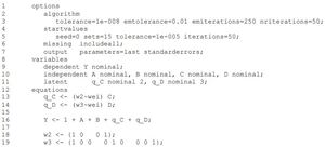
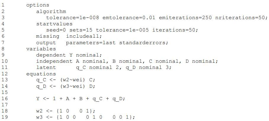
Figure 7 illustrates code for a multinomial dependent variable of any level with four independent variables: A and B are complete and are multinomial of any level, C is an incomplete 2-level multinomial variable, and D is an incomplete 3-level multinomial variable. Applying Fuchs’ approach to the independent variables requires the use of quasi-latent variables: a quasi-latent variable is a latent variable used to define a single manifest variable. In LG, latent variables can be specified on either side of an equation, but manifest variables can only be used on one side (independent variables on the right side; dependent variables on the left side). In our five-variable example, above, to fit a model for Y where C and D have been estimated using FIML techniques rather than mean imputation, independent variables C and D must be modeled in a latent framework. This is done by specifying categorical latent variables (line 11) and equations (lines 13 and 14) in Figure 7. The use of the weight statement (w2~wei and w3~wei) on lines 13 and 14 preserves the observed values. Weight equations are always specified at the end of the equations section (see line 18). LG by default applies Fuchs’ FIML estimation to variables on the left side of an equation. These FIML-estimated values for C and D are then used in the regression formula on line 16 to model Y using Fuchs’ FIML approach. This process is repeated in an iterative estimation-maximization fashion until convergence is reached for each model specified.

Figure 7.Fuchs-Fuchs model syntax in Latent GOLD 5.0

To use Fay’s approach in LG, response indicators must be added to the dataset for all variables with item nonresponse where Fay’s FIML approach is desired. In Figures 8 and 9, only the dependent variable is modeled using Fay’s approach; the response indicator for the dependent variable (iY) is added to the variables section on line 9. In Figure 8, the missing values on independent variables C and D are imputed via the default mean imputation. In Figure 9, these values are estimated using Fuchs’ FIML approach. Notice on line 14 of Figure 8 and line 18 of Figure 9 that iY is dependent on the structural variables A and B only. Under the MAR assumption, the model for iY can depend on any of the complete structural variables other than Y. Therefore, several response pattern models can be defined to model iY. The estimates of the structural model and the response models are influenced through the error terms; thus, various MAR response models should result in similar parameter and variance estimates for the model of Y.

Figure 8.Fay-Mean (MAR) model syntax in Latent GOLD 5.0

Figure 9.Fay-Fuchs (MAR) model syntax in Latent GOLD 5.0

Similar to Fuchs’ approach, Fay’s approach can also be applied to the independent variables through the use of quasi-latent variables. For the five-variable example, consider response indicators R, S, and T, which take on values of 1 when the variable is observed and 2 otherwise for variables Y, C, and D, respectively.

Models with more than one variable for Fay’s method are more complicated. Every variable with missingness for which Fay’s method is desired must have a response indicator on the dataset. These response indicators are added to the dependent line of the variables section (line 9 of Figure 10). Next, quasi-latent variables for each dependent variable and its response indicator that are needed on both sides of an equation must be specified on the latent line (line 11). Unless the joint distribution for the response indicators is known, each response indicator must be modeled separately.

The equation section begins by estimating the quasi-latent independent variables using all complete independent data. The equations for the quasi-latent variables must be defined working from least amount of missing to most amount of missing. Note that on line 14 the equation for the quasi-latent D variable contains the quasi-latent C variable. After line 13, all values for quasi-latent C are estimated. After all quasi-latent independent variables are estimated, the model of interest (Y) can be specified using all variables. Following Fay’s instruction, the response indicators are specified and modeled after the model of interest. In Figure 10, starting on line 18, the missingness of Y is dependent on A and B; the missingness of C is dependent on A; and the missingness of D is dependent on B. Again, several MAR models could be specified here. Lines 22 to 25 connect the quasi-latent variables to the observed data. When this set of equations is estimated at the same time using estimation-maximization techniques, Fay’s FIML approach is applied to both the independent and dependent variables with a MAR response mechanism.

Figure 10.Fay-Fay (MAR) model syntax in Latent GOLD 5.0

Modeling Assuming Data Missing Not at Random (MNAR)

Extending Fay’s MAR application to MNAR is straightforward. Under a MNAR response mechanism, the missingness of a variable depends on the variable itself; see Figure 11.

Figure 11.Missing not at random (MNAR) model path diagram

Consider the case of the Fay-Mean MAR application in Figure 8. To convert this model to a MNAR model, line 14 must be modified by adding Y to the dependent side. Since Y must now be used on both the independent and dependent sides of separate equations, a quasi-latent variable for Y must be created. By creating a latent variable for Y, we can now use the unobserved latent value of Y to predict the response probabilities and the observed values of Y. Therefore, the MNAR code for a Fay-Mean model looks similar to Figure 12. Note this is the simplest MNAR response pattern, but other response patterns can be specified. Similar modifications allow Fay’s FIML application to model MNAR for the dependent variables as well. Fay’s method can be mixed with Fuchs’ method.

Figure 12.Fay-Mean (MNAR) model syntax in Latent GOLD 5.0

Discussion

This report demonstrates how to fit FIML models that compensate for item nonresponse in categorical data analysis using Latent GOLD 5.0. Here we consider and contrast the two approaches (Fuchs’ and Fay’s) and discuss a few noteworthy results that emerged.

Implementing Fay’s method in LG presents a few unique challenges. Applying Fay’s method to only one variable in the model with LG requires the creation of a response indicator, two quasi-latent variables, and four equations. When missingness for more than one variable is being modeled, the addition of these variables and equations can result in models that sometimes do not converge. Specifically, the models invoking Fay’s FIML approach on all variables may produce convergence warnings regarding boundaries and rank deficiencies. These warnings may be the result of the additional response indicators, quasi-latent variables, and equations required to apply Fay’s approach in LG, which may indicate models with questionable stability. In some cases, Bayes smoothers can be used to resolve these warnings; directions for implementing Bayes smoothers in LG can be found in the technical manual.

An important advantage of the ability to fit MNAR models is to test whether missingness for one or more variables is MNAR or MAR. The appropriate missing data mechanism can be tested by visually comparing estimates from MAR and MNAR models; when estimates differ significantly between the two methods in either direction, then a MNAR nonresponse mechanism may be present. The disadvantages of treating item missingness as MNAR are larger variances and increased model complexity, which can lead to model instability due to weak identifiability and local minima (Bartolucci et al., 2013; Biemer, 2011).

It is possible that not all variables in a model are subject to the same missing data mechanism. Given the flexibility of LG, the code demonstrated in this methods report may be adjusted to model a mix of FIML MAR and MNAR approaches. Mixing these techniques might produce better estimates, but the impact on complexity, variance, and burden of fitting such models must be considered.

In conclusion, these FIML techniques are best used as a set. When MAR and MNAR FIML models are fit to categorical data, the nature of the missing data mechanism can be identified through model comparison. Given the potential difficulties of coding and fitting Fay’s response indicator models in LG, we recommend using LG’s default procedure that uses Fuchs’ approach whenever a MAR mechanism seems appropriate based on visual comparison of the estimates and fit statistics of the considered models. However, Fay’s response indicator approach is currently the only choice for fitting MNAR models in LG. For testing whether missingness is MNAR or MAR, Fay’s method should be used—but for best results, use it on the MNAR variable. Fitting various models under MNAR and MAR nonresponse mechanisms is recommended to identify variables with missing data that are MNAR. This approach will also identify when MNAR models produce invalid estimates due to either model convergence errors or software coding errors.

Acknowledgments

The authors would like to thank NSF for sponsoring this research. However, we would like to note that the views expressed in this paper are those of the authors only and do not reflect the view or position of NSF or RTI.