Cyclical Tree-Based Hot Deck Imputation

Introduction

Item nonresponse in survey data is common, especially in a large, complex survey in which the missing values might be caused by either the complexity of the questionnaire structure (e.g., skip patterns), difficulty of the topics in the survey items (e.g., sensitive topics, difficult concepts or data requiring access to information, files, or documents somewhere), data inconsistencies that lead to “blanking out” during the editing process, or some other unknown cause. When respondents with missing values are different than respondents that reported values, any analysis that is based on reported values only and does not account for the missing values may induce bias in the estimates (i.e., nonresponse bias). Even if the estimates are not biased, they probably have lower precision than estimates in which the missing values do not exist, usually because of smaller sample size. Item nonresponse also raises the concern that the variance of the statistics may also be biased.

In this report, we consider a survey that collects data on multiple variables, some of which have missing values. A common method to deal with item nonresponse is to impute these missing data. Imputation, if done properly, can reduce potential bias due to missing values. Imputation allows for data analysis based on complete data as if the data had no missing values; data that do not use imputation, however, commonly have cases with missing values dropped from the analysis. Hence, imputation may improve precision of the estimate by maximizing the sample size for data analysis.

One popular imputation method, especially for large, complex survey data, is hot deck imputation, which is a method that fills in a missing value with a reported value from a respondent within the same data/survey. In the item nonresponse context, cases with missing values are the nonrespondents, and cases with reported values are the respondents. In hot deck imputation terminology, a nonrespondent is also called the recipient (of imputed data), and the respondent providing the imputed value is called the donor.

Hot deck imputation commonly includes two steps: (1) imputation class construction and (2) donor selection within the classes. The methods used to form imputation classes and to select a donor within the imputation class vary from one hot deck approach to another. When the missing values for an outcome variable (variable being imputed) are missing at random (MAR; Rubin, 1976)—that is, the missing value is independent of the value of the variable itself but dependent on other variables in the data—hot deck imputation of this outcome variable can take advantage of the correlation between this imputed variable and the other variables (covariates). This method of donor selection assumes that when the donor’s and recipient’s values of covariates are alike, the recipient’s and donor’s outcome variables are also alike. For this reason, respondents and nonrespondents are grouped into homogeneous classes (called “imputation classes”) based on their observed covariates.

At this step, the imputation classes may also be sorted by additional covariates to add another level of granularity of the “match” between donor and recipient within an imputation class (i.e., “implicit” imputation classes). Sorting variables are often added when including these variables in the construction of explicit imputation classes might create imputation classes that have no donor. Once the imputation classes are formed, a donor is selected from within the same imputation class as the recipient.

Because every imputed value in hot deck imputation comes from valid reported values from respondents within the survey, conceptually, hot deck imputation should guarantee plausible imputed values that exist within the distribution of realized sampled values in the survey data. In this context, the hot deck method is a nonparametric method of imputation, whereas alternative imputation methods that use imputed values generated or predicted based on an explicit model are categorized as parametric imputation methods (Honaker et al., 2011; Raghunathan et al., 2001; Schafer, 1997; Yuan, 2011). There is also a hybrid (semi-parametric) imputation method in which the predicted values are computed based on an explicit predictive model, but these values are not used as imputed values. Instead, predicted values are used to match the respondent and nonrespondent to get the donor values; for example, predictive mean matching (also known as predictive mean neighborhood) can be used (Little, 1988; Rubin, 1986).

When imputing multiple correlated variables, the imputer has options to jointly model this vector of variables to be imputed using a multivariate distribution (i.e., joint modeling approach) (Honaker et al., 2011; Schafer, 1997) or to model each variable individually (i.e., sequential imputation approach) (Raghunathan et al., 2001; van Buuren et al., 2006; van Buuren & Groothius-Oudshoorn, 2011). In practice, with large survey data with several types of variables, under the joint modeling imputation approach, the imputer may not be able to account for correlation among variables with different types and distributions under one imputation model. However, with the sequential approach, correlation across imputed variables can be handled by fully conditional specification where once a survey variable has been imputed it can be used as a predictor in the model for imputing the next variable in the sequence. The differences in the approaches used in hot deck lead to different names/terms for these hot deck methods. Andridge and Little (2010) provide a comprehensive review of several hot deck methods.

In this report, we present a multivariate hot deck imputation approach called the Cyclical Tree-Based Hot Deck (CTBHD) for complex survey data commonly characterized by a large number of variables, different types of variables, a large number of categories in some categorical variables, a complex relationship structure of variables including skip patterns and compositional variables, and nonmonotone missing patterns, such as a “Swiss cheese” missing data pattern (Judkins, 1997). A system proprietary to RTI International, CTBHD incorporates several features that already exist in imputation work. CTBHD was developed to handle:

• a large number of variables to be imputed;

• a large number of candidate covariates for class and sorting variables and variable selection from this large number of variables;

• preserving associations among survey variables, including skip patterns;

• power issues when performing regression using a large number of predictors with a limited number of observations (e.g., because of a high missing rate);

• small sample sizes or no donor issues in imputation classes;

• vector imputation for compositional variables to avoid anomalous variable combinations in the imputed data; and

• repeated or cycled imputation for all variables with the goal of establishing stability in the imputation.

Imputation software for multiple variables has been available for some time and can address some of these needs. However, when relationships among variables are too complex, this software may not be able to handle such complexity without user customization of the imputation process. CTBHD is set up to allow the user to construct imputation classes based on user prior knowledge (“subjective” inclusion), data-driven inclusion based on empirical learning data, or a mix of the two. For the data-driven approach, CTBHD implements a statistical method in which class variables are statistically selected by the classification and regression tree (CART) approach (Breiman et al., 1984; Ripley, 1996).

Some survey variables to be imputed could be a type of compositional variable in which several variables correlate in the sense that the values of these variables are constrained by restrictions forming dependency (Judkins et al., 1993). A simple example of compositional variables is when a survey collects variables on the total number of household members (variable $Y_{1}$) broken down by age group—for example, 0–18 (variable $Y_{2}$), >18–60 (variable $Y_{3}$), and >60 (variable $Y_{4}$)—where $Y_{1} = Y_{2} + Y_{3} + Y_{4}$. An example of a case with missing data would be if two of these four variables are missing and none of the missing values can be filled in by deduction (subtraction or addition). In such a case, imputation has to deal with a vector of variables imputed at once, and the values are constrained by the specific edit rule that exists among these variables. In hot deck vector imputation, by default the reported values among the variables in the vector are preserved (instead of being replaced by donor’s values), and only the missing values among the variables in the vector are imputed. If there is no constraint or edit rule, then this set of compositional variables can be imputed as the “whole vector” imputation, without taking into account the reported values in the recipient. If there is a constraint, vector imputation may lead to an implausible outcome of imputed values because it violates the constraint/rule. In this case, the imputation requires a specific algorithm, which we explain in a later section about imputation of compositional variables.

In addition, for donor selection within the imputation classes, CTBHD incorporates the survey weights by implementing the weighted sequential hot deck (WSHD; Cox, 1980; Iannacchione, 1982). WSHD was developed based on the goal that the survey weighted mean and proportion estimates computed based on the WSHD imputed data will be equal, in expectation, to the weighted mean and proportion estimated using respondent data only. The methodology section gives further details on WSHD.

An additional variation of hot deck imputation (although it does not necessarily pertain to the hot deck method only) is to cycle the imputation process several times; that is, the same process to produce a set of imputed data is repeated (say C times), where when imputing a variable in cycle c, any imputed values resulting from the previous cycle (cycle $c - 1$) are used as if they were reported values. The final imputed values (a final dataset) come from the last cycle of imputation. Cycling the imputation is also carried out in the multiple imputation approach proposed by Rubin (1987) to produce more stable imputed values with less bias and smaller variance.

One other feature in CTBHD is the ability to recode or edit variables “on-the-fly.” This is an option that can be useful in several situations caused by edit rules based on one-to-one logical relationship among variables, including skip patterns. For example, if a gate variable is imputed with a “no” value, then the follow-up variable(s) that will be used as covariates in the next imputation step must first to be imputed or edited to “ineligible.” Another example is a derived variable used as a covariate in one imputation step that needs to be recreated based on the components computed in the previous step. The Methods section presents details of methods and features implemented within CTBHD.

Several authors have investigated asymptotic theory of properties for specific hot deck imputation under specific conditions; see for example, Rao and Shao (1992); Rao (1996); Chen and Shao (1999); Shao and Steel (1999); Brick, Kalton, and Kim (2004); Haziza and Rao (2006); Yang and Kim (2019). The development of the CTBHD approach required investigating the properties of these approaches. However, the complexity of the methods, particularly the mix of several methods implemented and the inclusion of several features within CTBHD, makes deriving the asymptotic properties of the CTBHD approach challenging, if not impossible.

In this paper, the performance of the CTBHD imputation system is evaluated through an empirical simulation study. In the Simulation section, we present our simulation based on the preliminary released (July 2022) microdata of the 2020 Residential Energy Consumption Survey (RECS) data available as a public use file from the Energy Information Agency of Department of Energy, which is the sponsor of RECS. In the last section, we present conclusions and discussion.

Methods

Notations

Let $\mathbf{Y} = (Y_{1},Y_{2},\cdots,Y_{k})$ denote variables that are subject to nonresponse, and $k$ denote the total number of variables that will be imputed. Further, let $\mathbf{X} = \left( X_{1},X_{2},\cdots,X_{p} \right)$ denote variables without missing values, and $p$ the total number of variables that will be used either as class or sorting variables. Note that in sequential multivariate imputation, when imputing a particular variable $Y_{i}$, the covariates for imputation classes or sorting variables may include members of $\mathbf{Y}$ (excluding $Y_{i}$) that have been imputed in previous steps of the imputation sequence, or in previous cycles. Thus, when a survey outcome variable within Y is included as one of the covariates but it has no missing values, we use notation $Y^{I}$ to denote the survey variable that has been imputed.

The missing pattern of $Y_{1},Y_{2},\cdots,Y_{k}$ can be nonmonotone, and the order of $Y_{1},Y_{2},\cdots,Y_{k}$ has not been determined yet. This is because $Y_{1},Y_{2},\cdots,Y_{k}$ can be ordered based on their missing rates from the smallest to the largest or can be ordered based on their order of appearance in the survey questionnaire. The latter is frequently used in situations in which a gate variable needs to be imputed before the follow-up variables. For all $i = 1,\cdots,k$, the goal is to impute missing values $Y_{i}$ fully conditioned on all observed values in $(\mathbf{Y}\mathbf{,}\mathbf{X)}$ except $Y_{i}$. For a specific variable $Y_{i}$ with some missing values, let $s_{r}$ and $s_{m}$ denote, respectively, the set of respondents and nonrespondents. Under hot deck imputation, reported values in $s_{r}$ (donors) will be used to impute missing values in $s_{m}$ (recipients).

Constructing Imputation Classes Using CART

For the construction of imputation classes in CTBHD, the default approach is to use a data-driven or “learning sample” approach that is based on the CART method to produce terminal nodes (Breiman et al., 1984). These terminal nodes then become the imputation classes. This is implemented using R package “tree” (Ripley, 1996). Given variable $Y_{i}$ to be imputed, the CART model defines $Y_{i}$ as the dependent (left-hand–side) variable, and $\mathbf{X}$ as the independent (right-hand–side) variable. CART can handle categorical variables (where a classification tree is produced) and continuous variables (where a regression tree is produced) for both $(\mathbf{Y}\mathbf{,}\mathbf{X)}$. Ordinal variables can be treated either way.

The CART process consists of the following steps:

1. Pick variable used for splitting.
2. Split data.
3. Repeat (a) and (b) until stop.
4. Predict/assign classes.

The construction of the tree deals with the selection of the splits, the decision to stop or to continue to split the node, and the assignment of a terminal node to a class. For imputing $Y_{i}$, a tree starts with a root node and is then grown from top to bottom by binary recursive partitioning using the respondent values of $Y_{i}$ in the specified model. Given $\mathbf{X}$ (variables with no missing values), the root is split first based on the most important significant variable, which maximizes the decrease of misclassification/“impurity” (measured either based on Gini index for classification trees or deviance for regression trees). At each internal node in the tree, this method applies a test to split the data. Of all possible splits, the split that produces homogeneity within the group and maximizes the reduction in misclassification rate is chosen, the data are split, and the process is repeated.

Continuous variables are divided based on a cutoff value a: X < a and X ≥ a. For categorical variables, the levels of an unordered factor are divided into two nonempty groups. No categorical variable can have more than 32 levels. Because a classification tree involves a search over (2^(d-1)-1) groupings for d levels, tree growth is limited to a depth of 31. In practice, however, this limitation will depend on the size of the dataset and computer performance; hence the number of maximum categories that can be handled may be lower than 32 levels. If a categorical item has too many levels, the tree program may crash or stop. In a situation in which a categorical variable has more than 31 levels, the user, prior to running CTBHD, needs to recode the categories to 31 or fewer categories based on some (subjective or informed) prior knowledge.

The tree stops growing when the current node is smaller than the user-provided value of minimum node sample size (“minsize”) or when one of two nodes that would be created by a split of the current node is smaller than the user-provided value of “mincut.” Usually, minsize = 2 × mincut. The terminal nodes become the imputation classes, where within a class, response values $Y_{i}s$ will be used as potential donors for the nonrespondents.

Because the tree is constructed based on the respondent cases, it is still possible that the regression tree produces imputation classes that have the minimum number of respondents but also have a large number of nonrespondents. In this case, a particular respondent might be overused as donor, or there may not be respondents with $\mathbf{X}$ data corresponding to the nonrespondent’s $\mathbf{X}$ data, resulting in an imputation class without a donor. The CTBHD system includes a feature that reports the number of times a donor is used. It will also stop the imputation process when encountering an imputation class without a donor. In these situations, the simplest solution is usually to increase the value of mincut.

Nevertheless, the use of CART to form imputation classes has an advantage over the traditional, complete cross-classification of covariates. In the regression tree, the nodes/cells are formed only when the variable levels/categories are statistically significant, whereas in complete cross-classification, all combinations of levels are used to form potential cells, some of which may have a small number of cases. In such a case, cells may be collapsed, either in an ad hoc or subjective manner or by prespecified rules. In a regression tree, the splits are done based on formal statistical tests, which do not require prior knowledge or assumptions. Note, however, that the “tree” program does not use weights when forming imputation classes. There is a weight option available in the tree command. However, we have not used this option, yet. While the use of weights may improve the tree construction, it could lead to more imputation classes with a small number of donors. This is something we would like to explore in future research because it will require using a different simulation study.

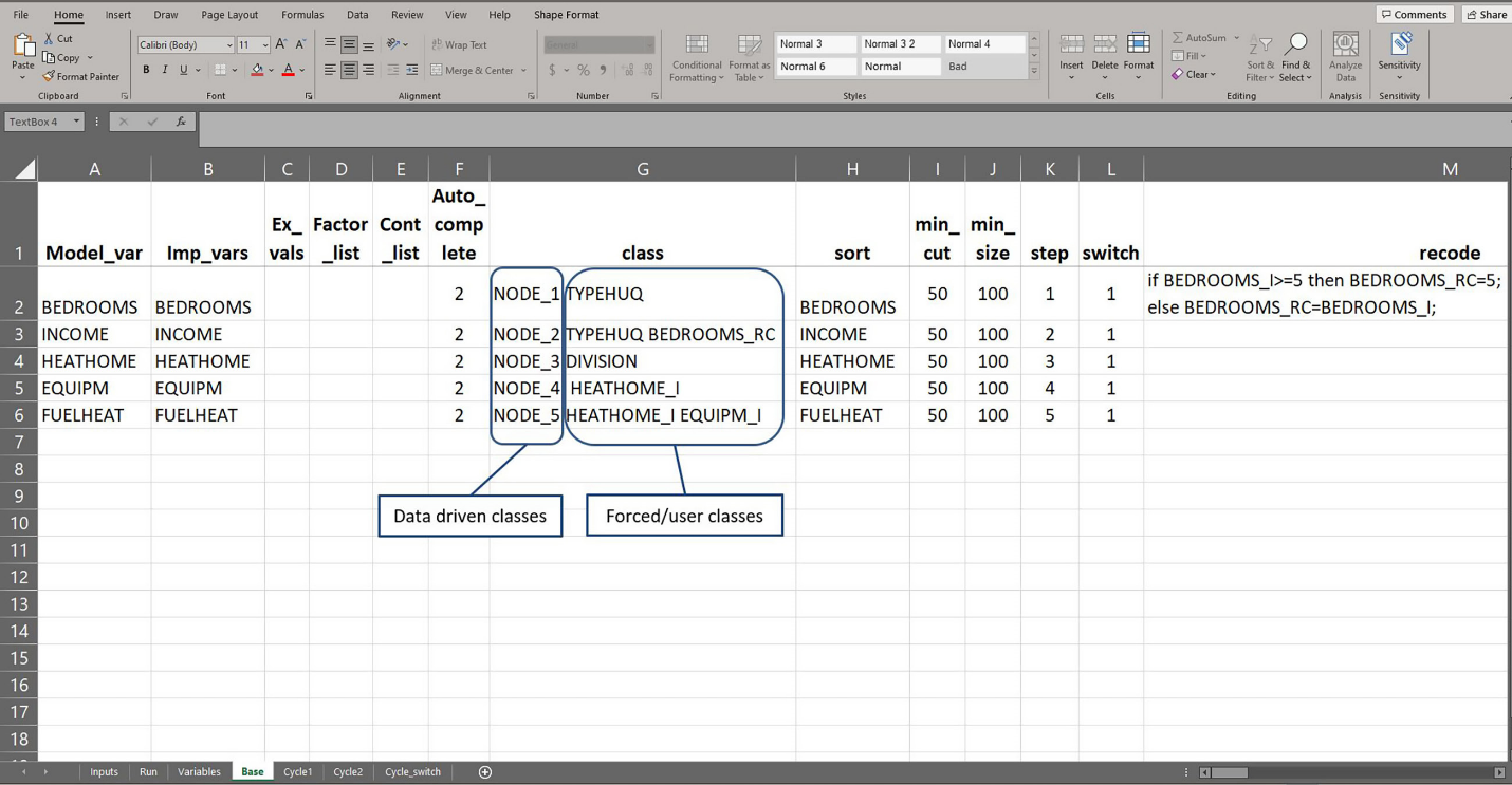
In addition, these terminal nodes from CART can be combined with classification variables known to be correlated with the variable being imputed (we call these “forced” class variables). We cross the categories of these forced class variables with the terminal nodes from the tree to form the final imputation classes (see an example of implementing the forced class variables in Figure A4 in the appendix). Crossing forced variables with the terminal nodes from the tree ensures that variables believed to be strong predictors (or “control” variables) are included in final imputation classes. This is why the crossing takes place after the terminal nodes are produced by CART, instead of running CART within each class defined by forced variables, which would complicate the computation.

Donor Selection: Weighted Sequential Hot Deck

When the data comes from a nonsimple random sample or weights are needed to get unbiased estimates from these data, ignoring the weight in selecting a donor would lead to biased imputed estimates. For example, for a simple single imputation class with uniform response mechanism and a simple random sampling to select a donor, the following estimate ${\widehat{Y}}_{i}$, computed based on imputed data,

$${\widehat{Y}}_{i} = \sum_{j \in s_{r}}^{}{w_{j}Y_{ij} +}\sum_{k \in s_{m}}^{}{w_{k}Y_{ik}^{*}}$$

will be biased, where $s_{r}$ is the set of respondents (donors), $s_{m}$ is the set of nonrespondents (recipients), $w$ is the survey weight, and $Y_{ik}^{*}$ is the imputed value, which is a reported value or donor from $s_{r}$. An alternative approach is to adjust the imputed value based on a reported value to produce an unbiased estimate ${\widehat{Y}}_{i}$. However, this approach is not practical because the unbiased property is valid only for a specific estimator. An idea for overcoming this bias issue is to use the survey weight in selecting a donor; that is, by choosing a donor $Y_{ik}^{*} = Y_{ij}$ with probability $w_{j}/\sum_{{j \in s}_{r}}^{}w_{j}$, where $Y_{ij}$ and $w_{j}$ are the reported value and the weight for donor $j$ from $s_{r}$, respectively. This approach will result in an unbiased estimate (see Rao & Shao, 1992, for proof). Cox (1980) provided analytic proof that the survey weighted mean and proportion estimates computed based on the WSHD imputed data will be equal, in expectation, to the weighted mean and proportion estimated using respondent data only.

Under the WSHD, within an imputation class, $s_{r}$ and $s_{m}$ can be thought of as two separate files (one file of respondents and one of nonrespondents). Both have survey weights attached to each case. The WSHD imputation process uses weights to “match” donors to recipients within an imputation class. Cases in $s_{r}$ need to be sorted based on $Y_{i}$ (see example of implementing this sorting in Figure A4 in the appendix), while cases in $s_{m}$ can be sorted randomly. For a categorical variable $Y_{i}$, donors having the same level are listed together. Let $\left\{ w_{1},\cdots,\ w_{r} \right\}$ denote the corresponding set of survey weights of sorted respondents, and $\left\{ v_{1},\cdots,\ v_{m} \right\}$ denote the corresponding set of survey weights of sorted nonrespondents. The nonrespondent’s weight $v_{k}$, $k = 1,\cdots,m$, is rescaled to:

$$s_{k} = v_{k}\frac{w_{+}}{v_{+}}\ ,$$

where $w_{+} = \sum_{{j \in s}_{r}}^{}w_{j}$ and $v_{+} = \sum_{{k \in s}_{m}}^{}v_{k}$.

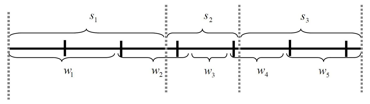
Then, the weights $\left\{ w_{1},\cdots,\ w_{r} \right\}$ are cumulated and partitioned into $m$ zones of length $\left\{ s_{1},\cdots,\ s_{m} \right\}$. When missing values (recipients) and reported values (donors) are expanded sequentially by their weights, these can be viewed as two matched files that cover the range from zero to the sum of the weights. The recipient range is essentially partitioned into $m$ zones, where each zone corresponds to the magnitude of a recipient’s adjusted weight $s_{k}$. For illustration purposes, Figure 1, copied directly from the SUDAAN Manual (Research Triangle Institute, 2012), presents an example of three donor selection zones assuming three item nonrespondents/recipients with associated weights $s_{1},s_{2},s_{3}$, and five donors with associated weights $w_{1},\cdots,\ w_{5}$.

Figure 1.Visualization of WSHD donor selection with three recipients and five donors

Source: Research Triangle Institute (2012).

The WSHD imputation algorithm finds a donor for each missing value from the potential donor(s) whose weights are in the corresponding zone on the donor range. When a zone has more than one donor, the recipient receives an imputed value randomly selected from the multiple donors. For example, based on cases in Figure 1, the donor for the recipient corresponding to weight $s_{1}$ will be randomly selected from cases with corresponding weights $w_{1},\ w_{2}$; the donor for the recipient corresponding to weight $s_{2}$ will be randomly selected from cases with corresponding weights $w_{2},\ w_{3},\ w_{4}$; and the donor for the recipient corresponding to weight $s_{3}$ will be randomly selected from cases with corresponding weights $w_{4},\ w_{5}$.

This process is done within each imputation class, so that the expected unbiased property applies for each class. Another advantage of this approach is that the number of times a donor is used will be limited. Sorting or “sequential” selection guarantees that a single record will not be used excessively as a donor. For this paper, the WSHD was implemented using the SUDAAN procedure “IMPUTE” (Research Triangle Institute, 2012).

Sequential Imputation

As mentioned in the introduction section, CTBHD imputes $\mathbf{Y}$ through a sequential imputation instead of modeling them jointly. Sequential imputation here means that the individual $Y_{i}$, $i = 1,\cdots,\ k$, will be imputed one-by-one. To preserve the interdependencies in $\mathbf{Y}$, when imputing a variable $Y_{i}$, the previously imputed variables in $\mathbf{Y}$ are included as covariates along with $\mathbf{X}$. The sequence of imputation is as follows:

Step 1: impute $Y_{1}$ using candidate covariates $\mathbf{X}\mathbf{,}$

Step 2: impute $Y_{2}$ using candidate covariates $(Y_{1}^{I},\mathbf{X})$,

Step 3: impute $Y_{3}$ using candidate covariates $(Y_{1}^{I},Y_{2}^{I},\mathbf{X})$,

⁝

Step $k$: impute $Y_{k}$ using candidate covariates $(Y_{1}^{I},Y_{2}^{I},\cdots,Y_{k - 1}^{I},\mathbf{X})$,

where $Y_{i}^{I}$ denotes the imputed variable $Y_{i}$ from Step $i$, $i = 1,\cdots,k$.

In these notations, we have not specified what rule determined the order of imputation sequence for $Y_{1},Y_{2},\cdots,Y_{k}$. The order of variables in this imputation sequence will impact the sample size used in the imputation process because the imputation process uses only those cases with observed data (no missing values) in both the variable being imputed $Y_{i}$ and the covariates. To maximize the power in modeling, intuitively, the first variable being imputed is the variable with the least number of missing values. So, the order of $Y_{1},Y_{2},\cdots,Y_{k}$ can be arranged based on their missing rates from the smallest to the largest. However, some variables may have relationships in a particular order, such as variables with a skip pattern (a gate variable and its follow-up variable[s]). Alternatively, one can perform imputation by following the order of items in the questionnaire, where we first impute the gate variable before imputing the follow-up variables, because the response to the gate variable will determine the treatment of the follow-up variables (i.e., whether it needs to be imputed or logically assigned a value of “not applicable” or “skip”). Note, however, in a situation where the gate variable is a binary variable but missing, and the follow-up variable is nonmissing, the imputer must set a rule for whether this gate variable should be (logically) edited or (statistically) imputed. For the latter, however, the imputation under this sequential order would fail to include the most correlated variable, which is the follow-up variable, because the variable still has missing values and is not included as a covariate.

Sukasih et al. (2018) carried out an investigation, through a simulation study using the 2015 RECS public use file (PUF), into whether the sequence of imputing two variables with a skip pattern relationship (a gate and a follow-up variable) in the CTBHD imputation impacts the estimates of proportion computed in these two variables. The result was that the order of imputation does not matter when cycling is used, and cycling is needed when the missing rate is not trivial.

Cycling the Imputation

The imputation steps defined previously in the Sequential Imputation section describe the steps for a base cycle of imputation $\mathbf{Y}$ to produce $\mathbf{Y}^{\mathbf{I}_{\mathbf{0}}} = (Y_{1}^{I_{0}},Y_{2}^{I_{0}},\cdots,Y_{k - 1}^{I_{0}},Y_{k}^{I_{0}})$, which is the imputed version of $\mathbf{Y}$, where the superscript $\mathbf{I}_{\mathbf{0}}$ indicates the imputation at base cycle. CTBHD has a feature to repeat the imputation several times ($C$ times), with the goal to produce more stable imputed values. The imputation of variable $Y_{i}$ at the $c$th cycle, however, is done using candidate covariates from all $(\mathbf{X},\mathbf{Y}_{\mathbf{- i}}^{\mathbf{I}_{\mathbf{c*}}}\mathbf{)}$, where $\mathbf{Y}_{\mathbf{- i}}^{\mathbf{I}_{\mathbf{c*}}} = (Y_{1}^{I_{c}},\cdots,Y_{i - 1}^{I_{c}},Y_{i + 1}^{I_{c - 1}},\cdots,Y_{k}^{I_{c - 1}})$ denotes the union of the $i - 1$ variables imputed before $Y_{i}$ in the cth cycle, and the $k - \ i$ imputed variables imputed after $Y_{i}$ in cycle $k - 1$. The sequence (steps) of imputation at cycle $c$ is as follows:

Step 1: impute $Y_{1}$ using candidate covariates $(Y_{2}^{I_{c - 1}},\cdots,Y_{k}^{I_{c - 1}},\mathbf{X})$,

Step 2: impute $Y_{2}$ using candidate covariates $(Y_{1}^{I_{c}},Y_{3}^{I_{c - 1}},\cdots,Y_{k}^{I_{c - 1}},\mathbf{X})$,

Step 3: impute $Y_{3}$ using candidate covariates $(Y_{1}^{I_{c}},Y_{2}^{I_{c}},Y_{4}^{I_{c - 1}},\cdots,Y_{k}^{I_{c - 1}},\mathbf{X})$,

⁝

Step $k$: impute $Y_{k}$ using candidate covariates $(Y_{1}^{I_{c}},\cdots,Y_{k - 1}^{I_{c}},\mathbf{X})$.

The result from the Sukasih et al. (2018) simulation showed that cycling the imputation has a stabilizing influence on the imputed values. Cycling could also solve the issue, described earlier, that occurs when imputation order is based on the order of survey items in the questionnaire.

There is no clear-cut way to determine the optimal number of cycles in the imputation. Martin et al. (2017) carried out an empirical study using data from the 2015 RECS and imputed 31 variables of varying types using CTBHD up to 10 cycles. The results indicated that cycling consistently showed impact on the imputed values on these 31 variables in the first three to five cycles, but there were few or no changes in the imputed values after the fifth cycle. In addition, the result showed that cycling has most impact imputation of continuous variables and the least impact on imputation of binary variables. Note, however, that the Martin et al. (2017) empirical study was not a simulation study that replicated the missing data and imputation; instead, it was an empirical study based on one realization of data only.

Imputation of Compositional Variables

A set of variables is compositional if a certain relationship or edit rule exists for them and the rule has to be preserved in the imputed data. A simple example based on the number of household members is given in the Introduction section. Another example is a set of four binary 0/1 variables $\left\{ Y_{1},\ Y_{2},\ Y_{3},\ Y_{4} \right\}$ representing the type of foundation in a single-family house, where $Y_{1} =$ type of foundation is a crawlspace, $Y_{2} =$ type of foundation is a basement, $Y_{3} =$ type of foundation is a concrete slab, and $Y_{4} =$ type of foundation is other, with the rule/constraint: $Y_{1} + \ Y_{2} + \ Y_{3} + \ Y_{4} > 0$. This rule essentially means that a single-family house must have a foundation. In compositional variables, any combination of variables in the set can be missing, creating missingness patterns.

Note that in some missingness patterns, given the relationship in compositional variables, the missing variables can be deduced from the values of reported/nonmissing variables, while in others imputation is required. For example, in the example of number of household member variables $\left\{ Y_{1},\ Y_{2},\ Y_{3},\ Y_{4} \right\}$ and $Y_{1} = \ Y_{2} + \ Y_{3} + \ Y_{4}$, for a missingness pattern that is missing $Y_{3}$ only—for example, $\left\{ 10,\ 2,\ .\ ,\ 5 \right\}$, where “.” indicates a missing value—$Y_{3}$ can be edited to $Y_{3} = 3$. In another missingness pattern, say $\left\{ .\ ,\ 2,\ .,\ 5 \right\}$, however, the value of either $Y_{3}$ or $Y_{1}$ must be imputed first and then the other variable can be deduced by addition or subtraction. In some missingness patterns, the constraint may not be based on the whole variables but instead may be applied only to a subset of variables (“derived constraint”). For example, under the relationship $Y_{1} = \ Y_{2} + \ Y_{3} + \ Y_{4}$, for a case with missing values $\left\{ 10,\ 2,\ .\ ,\ . \right\}$, the imputed values for $\left\{ Y_{3},\ Y_{4} \right\}$ have to meet the constraint $Y_{3} + \ Y_{4} = 8$.

When a set of compositional variables has missing values, imputing them one-by-one may produce an implausible outcome that violates the constraint/edit rule. In the example of house foundations $\left\{ Y_{1},\ Y_{2},\ Y_{3},\ Y_{4} \right\}$, there is a possibility that imputing them one-by-one may result in an outcome that is not allowed—for example, $Y_{1} = 0$, $Y_{2} = 0$, $Y_{3} = 0$, $Y_{4} = 0$, which is a single-family house without a foundation. In addition, if the imputation approach does not take into account the reported values that exist among the nonmissing members of compositional variables, the imputation may also produce implausible outcomes that violate the constraint/edit rule. In the example of compositional variables of number of household members with data $\left\{ 10,\ 2,\ .\ ,\ . \right\}$, the reported values $\left\{ Y_{1} = 10,\ Y_{2} = 2 \right\}$ have to be kept (which is the default in the hot deck vector imputation); the imputation cannot simply use any donor, because there is a derived constraint $Y_{3} + Y_{4} = 8$. In this case, the hot deck approach needs to account for $\left\{ Y_{1},\ Y_{2} \right\}$ by defining imputation classes that include $\left\{ Y_{1},\ Y_{2} \right\}$.

In addition to constructing the imputation classes based on $\mathbf{X}$, when imputing compositional variables using hot deck, the imputation process includes partitioning the data based on missingness patterns, determining the sequence of imputation by missingness patterns, and identifying subsets of donors and cases excluded from imputation for each missingness pattern. Then imputation is carried out for each missingness pattern. When imputing variables from one missingness pattern, nonrespondents from the other missingness patterns within the same set of compositional variables are ineligible to be donors. The exception to this rule is that cases that have been imputed for a particular missingness pattern can be used as donors for the next missingness patterns in the sequence. An example of imputation of compositional variables is given in the appendix.

Incorporating Editing or Recoding On-the-Fly

Imputation of complex variables such as compositional variables requires the imputer to be able to perform editing on-the-fly. Unlike imputation of one variable, where the whole sample is split into nonrespondents and respondents, and all missing values are imputed in one step, when imputing compositional variables, the entire sample is split into subsets by missingness pattern, and within each missing pattern, cases are grouped into three groups (nonrespondents, respondents/donors, and excluded cases). The members of these three groups change from one step to another. Therefore, subsequent variables need to be derived or recoded to classify cases into these three groups before the next variable can undergo imputation. The CTBHD system has a feature in which the imputer can add extra SAS code to be executed after a step of imputation is done. These new edits in the data will be used for the next imputation step.

Another example of the use of on-the-fly editing or recoding occurs when the imputation runs into a situation where the program stops and produces an error message (e.g., due to a no-donor issue) and imputation classes need to be collapsed. Two solutions for this situation are to drop the variable that creates sparsity from the imputation class variables, or to collapse categories in the variable that creates sparsity. When collapsing categories, a recoded variable could be created in the input data before imputation begins, or the imputer could collapse only the class that does not have a donor with an “adjacent” class. In the latter, this requires recoding a specific imputation class, so the collapsing is not done globally. This requires software that is capable of executing a cell-collapsing algorithm on-the-fly to avoid unnecessarily dropping/collapsing too many cells, which could introduce bias.

As a final, simple example, the most needed on-the-fly recoding occurs when a missing value in a gate/parent variable is imputed with a zero or “no”; then the follow-up variable can be immediately edited to “not applicable” or “skip”, so the skip pattern relationship is correctly coded for the next imputation step (see an example of a setup for an on-the-fly edit in Figure A4 in the appendix).

Simulation

For this paper, the CTBHD imputation is evaluated using an empirical simulation. The simulation used the 2020 RECS PUF that has 18,496 observations and is available for download from the US Department of Energy, Energy Information Agency (EIA) website (US Energy Information Administration, n.d.). The goals of this simulation are to evaluate the bias and root mean squared error of the estimates after imputing missing values using CTBHD and to demonstrate the performance of CTBHD. For comparison purposes, we ran imputation using other software that implements similar approaches to CTBHD. There are two freeware packages that implement similar imputation with regards to sequential/fully conditional specification and cycling approaches, namely, IVEware (Raghunathan et al., 2001) and MICE (van Buuren, 2018; van Buuren & Groothius-Oudshoorn, 2011). However, we specifically carried out the simulation to evaluate how the software handles imputation for variables with a skip pattern relationship. Skip patterns are handled in CTBHD in a semi-manual way: the user explicitly specifies the skip pattern relationship through the use of forced class variables. Neither IVEware nor MICE can directly incorporate skip pattern features as carried out within the CTBHD without specific program development.

For the imputation of variables with skip patterns with software that implements a predictive parametric model for imputation, such as in IVEware and as an option in MICE, these constraints can be handled only if the model includes all interaction terms for all variables involved in the skip pattern. Because a skip pattern is specific to only a small subset of variables within $\mathbf{Y}$, it is not clear how a skip pattern relationship that appears only among a subset of variables is applied in parametric modeling. Although MICE provides an option to use the CART method, it is unclear whether a skip pattern can be handled directly within the “mice” imputation command unless the user explicitly specifies imputation classes representing the skip pattern and then runs imputation “mice” command/model individually within these imputation classes. IVEware has an option to specify a skip pattern through the “RESTRICT” command; however, it is our understanding that the restriction creates only a binary class (two groups). It may not handle a restriction defined as cross-classification of categories in the variable being imputed and the covariate—for example, certain categories in the gate variable only go with certain categories in the follow-up variables. Nevertheless, we picked MICE for comparison with CTBHD because MICE provides a CART method for hot deck imputation classes.

The measure of empirical bias (EB) and root mean squared error (RMSE) will be calculated as follows:

• Empirical bias:
  $$EB = \frac{1}{R}\sum_{r = 1}^{R}\left( {\widehat{\theta}}_{r} - \theta \right)$$

• Root mean squared error:
  $$RMSE = \sqrt{\frac{1}{R}\sum_{r = 1}^{R}\left( {\widehat{\theta}}_{r} - \theta \right)^{2}}$$

where

$\theta$ = the true value for the outcome/variable of interest,

${\widehat{\theta}}_{r}$ = estimate of $\theta$ based on the r-th replicate of simulated data, and

$R$ = number of replicates.

The variables in RECS PUF include geographical and administration variables, survey variables (housing and household characteristics, energy bill and energy consumption related variables, etc.), and weights including analysis weight and replicate weights for variance estimation. For this simulation, we focused on a simple explicit skip pattern relationship among the following energy used (categorical) outcome variables HEATHOME, EQUIPM, and FUELHEAT:

• Space heating used (HEATHOME):
  0 = No, 1 = Yes

• Main space heating equipment type (EQUIPM):
  -2 = Not applicable (recoded to 0 for simulation)
  2 = Steam or hot water system with radiators or pipes
  3 = Central furnace
  4 = Central heat pump
  5 = Built-in electric units installed in walls, ceilings, baseboards, or floors
  7 = Built-in room heater burning gas or oil
  8 = Wood or pellet stove
  10 = Portable electric heaters
  13 = Ductless heat pump, also known as a “mini-split”
  99 = Other (recoded to 14 for simulation)

• Main space heating fuel (FUELHEAT):
  -2 = Not applicable (recoded to 0 for simulation)
  1 = Natural gas from underground pipes
  2 = Propane (bottled gas)
  3 = Fuel oil
  5 = Electricity
  7 = Wood or pellets
  99 = Other (recoded to 8 for simulation)

The following two covariates were included in the imputation simulation. The covariate DIVISION is a geographical variable representing Census division with values:

1 = New England
2 = Middle Atlantic
3 = East North Central
4 = West North Central
5 = Mountain North
6 = Pacific
7 = Mountain South
8 = West South Central
9 = East South Central
10 = South Atlantic

The covariate TYPEHUQ is a variable representing type of housing units as follows:

1 = Mobile home
2 = Single-family house detached from any other house
3 = Single-family house attached to one or more other houses (e.g., duplex, row house, or townhome)
4 = Apartment in a building with 2 to 4 units
5 = Apartment in a building with 5 or more units

True Value and Simulated Missingness

Missing values in the 2020 RECS PUF data have been imputed. In this report, we treat imputed data as if they were reported values (the “truth” for our simulation). The estimates of interest for our simulation are based on the table cells of Table HC6.1 (US Energy Information Administration, 2022), where the estimates are produced using the first version of 2020 microdata file released in July 2022 (see Table 1). These cells involve a skip pattern based on “uses space heating equipment” (variable HEATHOME), “natural gas” (variable FUELHEAT), and “central warm-air furnace” (variable EQUIPM), and a classifier “housing unit type” (variable TYPEHUQ).

The numbers in Table 1 are considered the true values for this simulation. From these data, we generated missing values. The simulation will demonstrate a nonmonotone MAR mechanism and a simple explicit skip pattern between HEATHOME as a gate/parent variable and child variables EQUIPM and FUELHEAT. That is, if HEATHOME = 0 then both EQUIPM and FUELHEAT are not applicable/skipped (EQUIPM = 0 and FUELHEAT = 0). In other words, only when HEATHOME = 1 then both EQUIPM and FUELHEAT are greater than 0.

We generated missing values assuming MAR as follows:

1. Missing HEATHOME depends on values of DIVISION, EQUIPM, FUELHEAT;

2. Missing EQUIPM depends on values of DIVISION, HEATHOME, FUELHEAT;

3. Missing FUELHEAT depends on values of DIVISION, HEATHOME, EQUIPM;

4. Joint missing (EQUIPM, FUELHEAT) depends on values of DIVISION, TYPEHUQ, HEATHOME.

For imputation modeling, we included two more variables with missing values (BEDROOMS and MONEYPY) that correlate with the variables of interest. These variables are included as potential predictors once their missing values are imputed.

BEDROOMS: Number of bedrooms (top-coded): 0–6
MONEYPY: Annual gross household income for the past year
1 = Less than $5,000
2 = $5,000–$7,499
3 = $7,500–$9,999
4 = $10,000–$12,499
5 = $12,500–$14,999
6 = $15,000–$19,999
7 = $20,000–$24,999
8 = $25,000–$29,999
9 = $30,000–$34,999
10 = $35,000–$39,999
11 = $40,000–$49,999
12 = $50,000–$59,999
13 = $60,000–$74,999
14 = $75,000–$99,999
15 = $100,000–$149,999
16 = $150,000 or more

It is common that in a simulation, values or missing values of a variable are generated using a specified model for that particular variable, and this is done one variable at a time. However, instead of generating missing values one variable at a time, we implemented a multivariate amputation procedure “amputation” provided in R package MICE (Schouten et al., 2018). The idea of this procedure is to control the joint missing rates and ensure that missingness follows the MAR assumption. Table 2 shows the summary of percentage of missing across 1,000 simulated data for each missing pattern shown in the first column of Table 2. The rates presented here do not reflect the real missing rates in the real RECS survey data.

We generated 1,000 replicates (R = 1,000) of simulated data with missing values in the three energy use variables HEATHOME, EQUIPM, and FUELHEAT.

Given the true values and simulated missing values generated under this procedure, based on the 1,000 simulated missing datasets, Table 3 shows the empirical bias of the estimates if someone used the data with missing values to calculate totals and proportions (complete case analysis in which the cases missing values were dropped). Because an estimate of total will have a negative bias if missing values are ignored (not imputed), in addition to calculating the estimate of total, Table 3 also shows the estimate of proportion of housing units that use natural gas and the proportion of housing units that use central warm-air furnace as their gas heating equipment, where the denominator for these proportions is the total number of housing units that use space heating equipment (HEATHOME = 1). Complete case analysis (without imputation) will incur nontrivial bias in both estimates of count and proportion.

Imputation and Evaluation

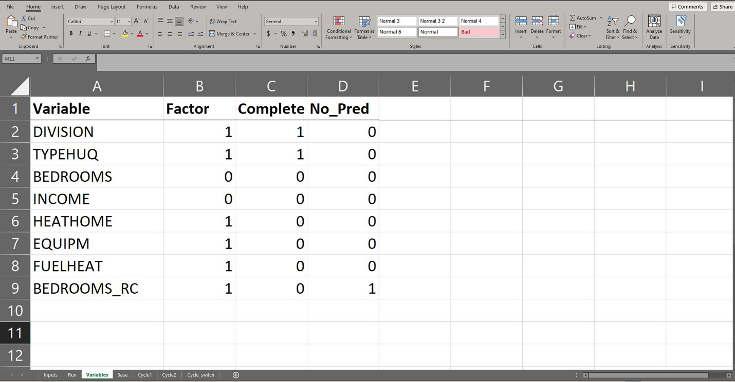
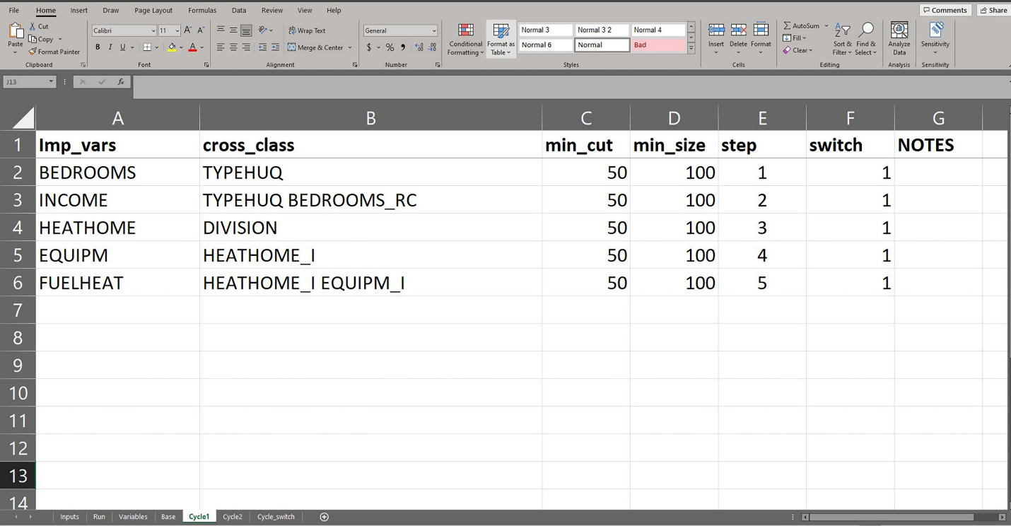
Under the CTBHD imputation we implemented the following imputation classes with values of mincut and minsize for the tree package as shown in Table 4. The suffix “_I” indicates a version of the variable that has been imputed in the previous step. For example, HEATHOME_I used as one of the imputation class variables in Step 4 no longer has missing values because those have been imputed in Step 3. The imputation variable “NODE_X” indicates the nodes resulted from CART approach produced in a particular step “X.” These classes/nodes given by “NODE_X” were data driven, whereas extra variables specified in addition to the “NODE_X” were the forced imputation classes crossed with “NODE_X” classes. This CTBHD imputation was run for three cycles (base, and cycles 1 and 2).

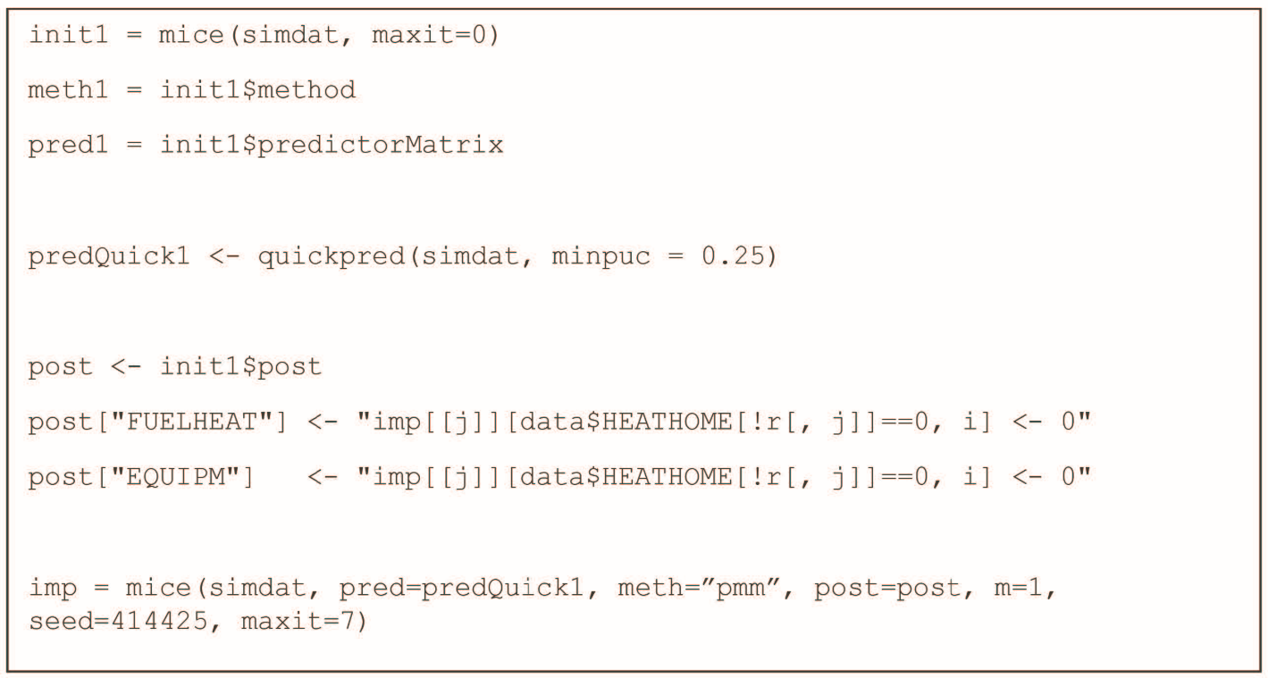
For comparison purposes, we also ran the imputation for the same simulated missing data using R package MICE under two imputation options: predictive mean matching (PMM) and CART. The R codes for MICE are shown in Figure 2.

Figure 2.R codes for MICE imputation

The codes in Figure 2 show R codes for MICE imputation based on a PMM approach. The codes for MICE that are based on CART can simply replace the “pmm” with “cart” in the parameter for method (i.e., meth=“cart”). By reviewing the predictors in the MICE models, we confirmed that similar variables used for imputation classes in CTBHD, as Table 4 shows, were also chosen as predictors for MICE models. Also note that in MICE, after imputation, we edited the imputed values of FUELHEAT and EQUIPM based on the outcome of HEATHOME; that is, if HEATHOME = 0 then FUELHEAT = 0 and EQUIPM = 0. This edit, however, does not need to be done in CTBHD because of the explicit use of HEATHOME as one of the imputation class variables.

Table 5 shows the result of the simulation in terms of EB and RMSE from imputation under the three approaches.

In general, when evaluating CTBHD performance by itself, the bias and precision of the estimates of totals are low. Comparing the MICE under PMM and CART to CTBHD, Table 5 demonstrates the performance of the three imputation approaches dealing with a multilevel conditional relationship (skip pattern) across variables. When imputing the root gate variable (i.e., HEATHOME), all three imputation approaches performed well with regard to bias and precision, and they are also relatively similar on the values of these measures. Note, however, upon checking the compliance on skip pattern rules between HEATHOME and FUELHEAT, and between HEATHOME and EQUIPM, the imputed values based on the PMM approach had some inconsistencies in which a few cases violated the HEATHOME-FUELHEAT edit rule and a handful of cases violated the HEATHOME-EQUIPM edit rule. This is because the PMM approach matched the donor and recipient based on covariates only implicitly through the model (which is essentially an imputation process based on a single imputation class), whereas the approaches based on CART in CTBHD and MICE CART used explicit imputation classes.

When it comes to imputing follow-up variables (FUELHEAT and EQUIPM), in general CTBHD performed better than the other two approaches with regard to bias and precision for all three variables and subdomains by housing unit type. MICE underestimated counts of single-family detached houses that used gas with central warm-air furnace by more than 1 million units. Its RMSE is also larger than that of CTBHD.

Conclusion, Limitations, and Discussion

When performing imputation of missing data in large, complex survey data, the imputer must consider several data factors including the volume of the data (number of variables and sample size), type of variables, missing mechanism, and structure of relationship among variables. In addition, the imputer has to choose the correct methodology and its corresponding computational resources. For this, CTBHD can handle imputation of missing values for many different kinds of variables and complex relationships across variables.

Either commercial/licensed software or freeware is available that is well developed based on general or specific method and purpose. With this software availability, the user/imputer must pick the software based on his or her need. When the software needed is not immediately available, the imputer has to develop his or her own. CTBHD is a hot deck-based imputation approach developed based on the need to impute missing values in large-scale, complex survey data with several types of variables that may have complex relationships, and where the imputer can have flexibility in defining imputation classes. CTBHD can also use weights in the imputation and cycle the imputation process.

We acknowledge that there are several algorithms/methods available for imputation class construction using classification and regression trees. CTBHD uses the CART algorithm that examines all possible binary splits of the data (exhaustive search method) and that is available through an R tree package. Variable selection in CART tends to choose variables that have more splits (see, e.g., Loh & Shih, 1997). To reduce potential variable selection bias in the CART algorithm, Loh and Shih (1997) suggest the QUEST (for Quick, Unbiased, Efficient, Statistical Tree) algorithm. When comparing QUEST and CART using two examples of data (simulated data and real data), Loh and Shih showed that the error rates from QUEST based on the simulated data are generally smaller than those from CART; however, the differences were small. Lin and Fan (2019) also evaluated CART, CHAID (for Chi-squared Automatic Interaction Detection), and QUEST and compared the accuracy of the three methods. They showed some different results in which the accuracy of CHAID was the highest, followed closely by CART, and the accuracy from QUEST was the lowest. Although they concluded that CHAID provided better results for their data, in our opinion, the difference was marginal, and the CART method is equivalent.

The work described in this paper evaluates performance of CTBHD through a large-replication empirical simulation for a subset of variables with a specific skip pattern relationship. It would be interesting, however, to see how CTBHD performs for other types of variables and their relationships—for example, compositional variables—starting from a simple constraint (e.g., the example of a single-family house foundation), a complicated deduction/subtraction/addition constraint (e.g., the example of the number of household members), or more complicated pairs of allowable outcomes (e.g., the edit rule between type of heating fuel and equipment; not discussed in this paper).

In hot deck imputation implementation, the imputer may often face a situation in which there is no donor available within an imputation class. Good software should handle this issue with a solution that could be automated or at least require minimum interruption in the whole imputation process and that is statistically valid. In CTBHD, this situation is handled by choosing one of several approaches that include increasing the sample size of the tree’s node, collapsing the particular node without a donor, or recoding the categories in the variable that creates the empty-donor class. In the current version of CTBHD, however, the user still needs to handle this solution manually.

Our simulation used MICE, a popular “canned” software, as a comparison to demonstrate how CTBHD and MICE handled item nonresponses in complex survey data. However, we realize that due to the limited capability of MICE programming, the comparison with CTBHD is not really apples to apples. For example, although both CTBHD and MICE CART use a CART approach for constructing imputation classes, the outcome of final imputation classes for each simulation replication may not be the same. CTBHD is able to include prespecified forced class variables for individual imputed variables, allowing the forced class variables to be different/customized across imputed variables. In MICE, the same prespecified forced class variables are used for all imputed variables. This reflects one of the limitations in using canned software. When there are few variables to be imputed, no missing patterns, and the relationships between variables to be imputed are simple, canned software may satisfy the user’s imputation needs. Many software packages are available for hot deck imputation, but again the user needs to know how the software implements the method, whether the software meets the imputer’s need, and whether a modification can be made to develop an imputation process (imputation class construction, donor selection, sorting variables, etc.) as needed.

Acknowledgments

The authors would like to acknowledge CTBHD system developers including Lance Couzens, Tommy Holder, Stephen Black, Jeremy Porter, and Darryl Creel; Phil Kott for suggesting the organization of the paper; and RTI Press reviewers for their helpful comments and suggestions.

The opinions expressed in this paper are those of the authors. They do not purport to reflect the opinions or views of RTI International nor the Department of Energy, Energy Information Agency, whose data are used for simulation study in this paper. Any errors are the fault of the authors.

RTI Press Associate Editor: Marcus Berzofsky