Introduction

Overview

Numerous research studies have shown that social, economic, environmental, political, and other non-medical factors play a large role in shaping health status (Braveman & Gottlieb, 2014). These factors have been found to account for 80 to 90 percent of a person’s health outcomes (O.’Neill Hayes & Delk, 2018). Social determinants of health (SDoH) are “the conditions in the environments where people are born, live, learn, work, play, worship, and age that affect a wide range of health, functioning, and quality-of-life outcomes and risks.” (Marmot et al., 2008) Implementing programs, policies, and investments that address differences in SDoH could help to improve the health of populations at high risk for serious illnesses and worse health outcomes (Baciu et al., 2017).

SDoH include both risk and protective factors. Income, for example, is a SDoH; associated measures and concepts can be both risk factors (e.g., poverty) and protective factors (e.g., wealth). Risk factors including poverty, racism, and housing insecurity are just a few of the nonmedical factors associated with poor health outcomes (Alderwick & Gottlieb, 2019; Muennig et al., 2010). Differences in SDoH and risk factors play a large role in shaping health disparities in the United States (Braveman & Gottlieb, 2014; Marmot et al., 2008). Disparities in health and SDoH are the metrics we use to measure progress toward achieving health equity and reducing health inequity (Braveman, 2014), which is defined as the systematic differences in the opportunities groups have to achieve optimal health, leading to unfair and avoidable differences in health outcomes (Baciu et al., 2017).

For decades, health and medical practitioners, researchers, and policymakers have called for a better way to measure, predict, and adjust for SDoH in healthcare and population health (Figueroa et al., 2020; Obermeyer et al., 2019). The goal of this work is to answer that call in a way that supports the achievement of health equity: attainment of the highest level of health for all people, where everyone has a fair and just opportunity to attain their optimal health regardless of race, ethnicity, disability, sexual orientation, gender identity, socioeconomic status, geography, preferred language, or other factors that affect access to care and health outcomes (Topchik et al., 2020).

We approached this research through the lens of risk adjustment for SDoH, also known as social risk adjustment. This manuscript outlines a novel approach to developing a health equity–focused index to expand risk adjustment models and demonstrates the utility of the measure in an analysis of a patient-centered medical home program in Ohio. We find that accurate multidimensional, cross-sector, small-area social risk scores could be useful in understanding the impact of healthcare innovations, payment models, and interventions on social drivers of health on high-risk communities; identifying neighborhoods and areas at highest risk of poor outcomes for better targeting of interventions and resources; and accounting for factors outside of providers’ control for more fair and equitable performance/quality measurement and reimbursement.

Background

Despite the enormous impact of SDoH on patient outcomes, current health system performance and quality measures generally do not consider SDoH, nor are SDoH generally included in most risk adjustment formulas (Ash et al., 2017; National Academies of Sciences, Engineering, and Medicine, 2017). Risk adjustment is a “statistical process that takes into account the underlying health status and health spending of the enrollees in an insurance plan when looking at their health care outcomes or health care costs.” (HealthCare.gov, n.d.) Risk adjustment is used in quality measurement and in calculating reimbursements to healthcare providers (Center for Medicare and Medicaid Services, 2021). Risk adjustment modifies payments to providers to account for differences in expected healthcare expenditures because of factors such as individual age, sex, and diagnoses (Irvin et al., 2020). This ensures that providers treating patients with higher risk (e.g., older patients) are paid more to treat such patients compared with those treating lower-risk patients. Risk adjustment is common in value-based payment (VBP) models, which provide payments to providers based on achievement of quality goals or cost savings as an important way to reduce incentives to care for only young, healthy, inexpensive-to-treat patients.

The Centers for Medicare & Medicaid Services (CMS) Innovation Center estimates that by 2030, 100 percent of people with Original Medicare (Parts A & B) will be cared for under a VBP model (Menzin et al., 2011). This reinforces the imperative that risk adjustment models accurately account for underlying individual- and community-level risk when predicting patient expenditures. In the zero-sum world of pay-for-performance and VBP models, omitting SDoH from risk calculations can lead to several unintended consequences. First, practices with patients who are at a lower risk of serious illnesses may receive rewards that reflect patient mix rather than quality, while practices with patients who are at a higher risk of serious illnesses may lose out on resources for improving quality (Guo & DuGoff, 2019; Lines & Sokol, 2020). Second, providers may object to being held accountable for factors outside of their control (Lines, 2018). Third, payers have incentives to enroll members with lower risk wherever possible, potentially leading to cream-skimming and cherry-picking (Bynum & Lewis, 2018). Finally, lack of good data on SDoH can lead to interventions targeting populations with a lower risk of serious illnesses, attenuating potential benefits from those interventions (Chen et al., 2020).

Previous work on social risk adjustment has employed analyses at the county or ZIP code levels or has approached measurement or risk adjustment for SDoH with factor analysis, principal component analysis, or simple weighted formulas (Flanagan et al., 2011; Singh, 2003). Several US small-area–based indices of social risk and socioeconomic deprivation are available, including the Area Deprivation Index (ADI), Social Deprivation Index (SDI), and the Social Vulnerability Index (SVI). These indices consider relatively few social factors and rely heavily on US Census data. Some of these indices are currently used in VBP models to increase equity in payments based on the area-level social risk factors of the population served. For example, the CMS Accountable Care Organization (ACO) Realizing Equity, Access, and Community Health (REACH) model uses the ADI to adjust ACO benchmarks based on the number of beneficiaries in the highest and lowest deprivation areas (Liao & Navathe, 2022).

The ADI, originally developed by Singh et al. more than 20 years ago (Singh, 2003), has been used in numerous studies to understand the association between neighborhood-level characteristics and health outcomes, such as hospital readmissions and expenditures (Liaw et al., 2018a; Raven et al., 2008). The ADI relies upon 17 socioeconomic indicators organized in four domains (income, education, employment, and housing quality), all of which come from the American Community Survey (ACS) 5-year sample at the Census block group level (Singh, 2003).

The SDI, developed by Butler et al (Butler et al., 2013). and maintained by the Robert Graham Center of the American Association of Family Physicians, is based on seven variables collected in the ACS at the Census tract level: (1) poverty rate, (2) adults without high school diploma, (3) percent single parent household, (4) percentage living in rented housing unit, (5) percentage living in overcrowded housing unit, (6) percentage of households without a car, and (7) unemployment.

The SVI (available at census tract and county levels), developed by the Centers for Disease Control and Prevention (CDC) and the Agency for Toxic Substances and Disease Registry, incorporates 15 Census variables, including poverty, lack of access to transportation, and crowded housing, within four domains: (1) socioeconomic status, (2) household composition, (3) race/ethnicity/language, and (4) housing/transportation. The SVI was specifically designed to understand social vulnerability in the context of natural disasters and emergency management (Flanagan et al., 2011).

The ADI (available at 9-digit ZIP code and Census block levels) (Singh, 2003) and SDI (available at county, census tract, aggregated ZIP Code Tabulation Area, and Primary Care Service Area levels) (Butler et al., 2013) were developed using factor analysis, a method with poor replicability over different space and time periods (Allik et al., 2020). In addition, the ADI is roughly 80 percent correlated with owner-occupied property values, which can be misleading. For example, the ADI rates neighborhoods with low homeownership rates as excellent when those few owned homes are very expensive, despite economic circumstances being difficult for most residents.

In this pilot study, we sought to develop a comprehensive neighborhood-level index to enable risk adjustment models to correct for inadequate adjustment for social risk factors. Although individual-level SDoH data are best for predicting individual-level outcomes, collecting this information can be difficult (Phillips et al., 2021). Area-level measures are associated with health outcomes and can be useful either in conjunction with individual-level data or on their own (Ash et al., 2017; Butler et al., 2013; Chang et al., 2021; Kind et al., 2014; Liaw et al., 2018b; Link & Phelan, 1995; Powell et al., 2020; Sapra et al., 2020).

We have developed an “artificially intelligent” approach to risk adjustment for SDoH using random forests (RFs) to understand life expectancy (LE) at the Census tract (CT) level. In the United States, LE inequality persists along racial, sex, and urban/rural lines (Sapra et al., 2020). Although LE has increased from a national average of 69.7 years in 1950 to 78.8 years in 2015, the averages vary dramatically across small geographic areas (Singh et al., 2017; Xu et al., 2016). For example, within Franklin County, Ohio, CT-level LE ranges from 60.0 to 87.6 years (Tejada-Vera et al., 2020).

Artificial intelligence (AI) is “a branch of computer science that explores the ability of computers to imitate aspects of intelligent human behavior, such as problem-solving, reasoning and recognition.” (Smith et al., 2020; Wellcome Trust, 2019) Machine learning (ML), an application of AI, is a popular tool in public health and health services research (Kino et al., 2021; Wiemken & Kelley, 2020). Researchers have used these tools in four different ways: (1) to predict an outcome Y based on a set of covariates X without ascribing any causal value to these covariates, (2) to identify bias in data and decision-making, (3) to enhance the evaluation of how treatment affects an outcome, and (4) to synthesize new data (Kino et al., 2021). For this paper, we focus on its pure prediction application via RFs. An RF model is a supervised ML model that creates multiple regression trees and aggregates their results with the purpose of forming a generalization about the relationship of covariates to the outcome of interest (Kaur et al., 2019). We used RF models to understand which SDoH variables explain the variation in LE at the CT level and to generate a composite SDoH measure, the Local Social Inequity (LSI) score, which is a ranked percentile score based on the RF-predicted outcome measure. Section 2 of the online Supplement provides additional background information about RFs (supplementary material can be found online at https://doi.org/10.5281/zenodo.7026658).

Aims

The aims of this research were threefold. First, we created a health equity–focused conceptual framework for risk adjustment of the SDoH. The framework provides context and rationale for the inclusion of SDoH variables and their links to our population health outcome, LE. We used LE at birth as our outcome measure because it is frequently used to measure the overall health status of a population (OECD, 2022). Second, we built upon our conceptual model to develop a health equity–focused index that comprehensively measures neighborhood-level social inequity. We used supervised ML and publicly available data to develop a new SDoH composite index that is robust, comprehensive, cross-disciplinary, spatially refined, and highly predictive. Finally, we pilot-tested the composite index in a patient-centered medical home program in Ohio and estimated associations between the index and individual-level core outcome measures for the evaluation: total expenditures, inpatient admission, hospital readmissions, and emergency department (ED) visit rates.

Methods

Conceptual Framework

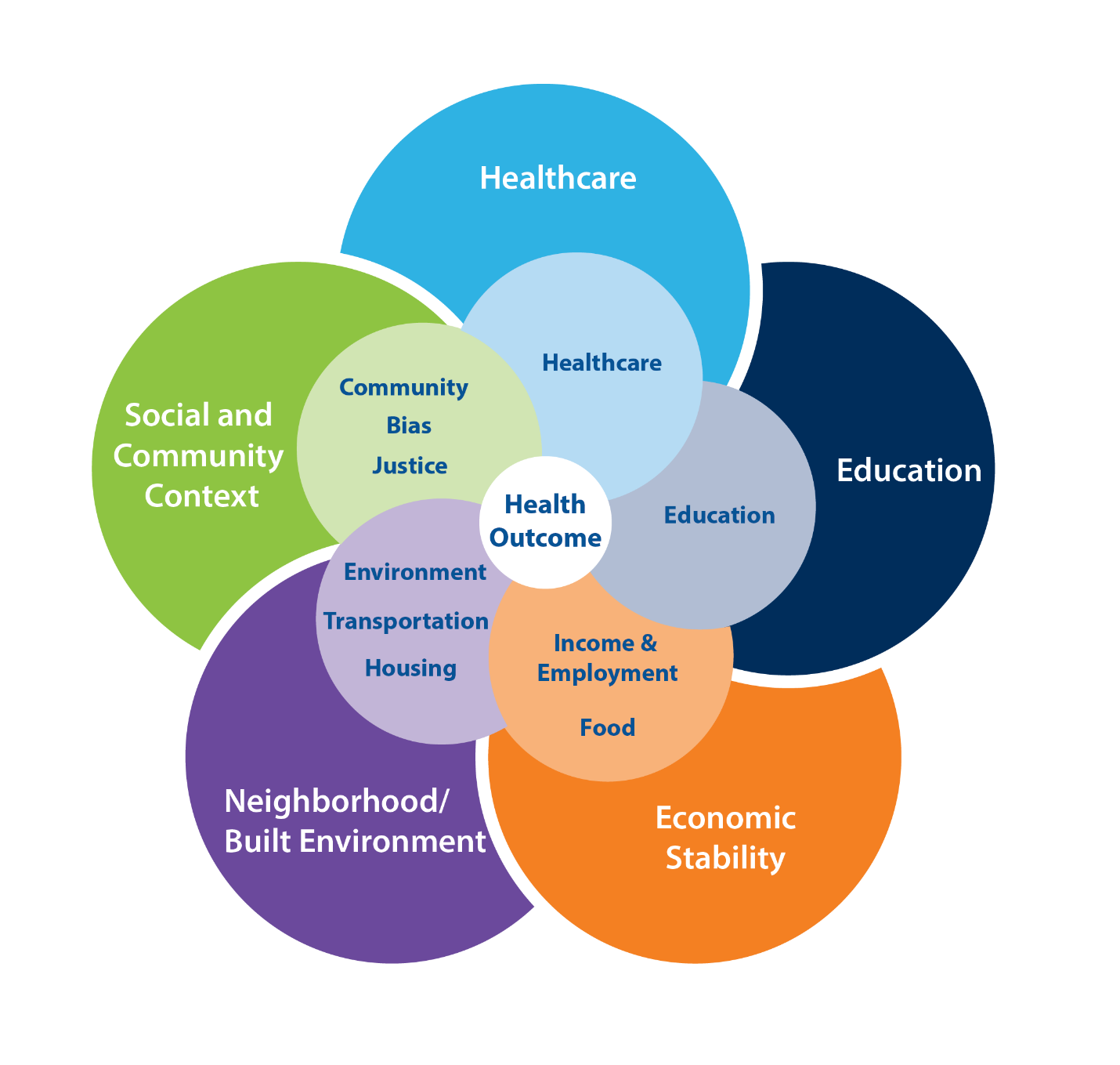
We started conceptualizing SDoH for this study by reviewing the literature on existing conceptual frameworks (Kilbourne et al., 2006; Marmot et al., 2008; Office of Disease Prevention and Health Promotion, 2020). We ultimately started with and then adapted the five domains in CDC’s Healthy People framework: healthcare access and quality; education access and quality; social and community context; economic stability; and neighborhood and built environment. We expanded these five domains into 10 domains, as follows, based on data and measure availability and potential associations with LE. First, we kept the CDC’s domains of (1) healthcare and (2) education. We expanded the social/community context domain to include three separate areas: community health, well-being, and healthy behaviors; bias, stress, and trauma; and justice, crime, and incarceration. We split the CDC’s economic stability domain into two: (1) food security and access to healthy food and (2) poverty, inequality, and employment. Finally, we expanded the neighborhood/built environment domain into three domains: (1) housing adequacy, crowding, and structural health; (2) environmental quality; and (3) transportation access, infrastructure, and safety. Figure 1 shows the domains at a glance and emphasizes their interconnectedness. The online Supplement Exhibit 1 provides the full list of measures from which the RF drew predictor variables in the main model and sensitivity analyses and rationales for inclusion.

Figure 1.Conceptual Framework: Social Determinants of Health

Addressing Bias

We addressed potential biases in our framework in several ways. First, we “tuned” our model to predict LE, because it is a high-level population health outcome that is commonly used in population health research. Second, we involved people in the development process from a variety of backgrounds and disciplines, bringing expertise and insights from multiple viewpoints—including people with direct experience with the social risks (e.g., food insecurity and poverty) we sought to measure. The team included staff with expertise in health services research, social epidemiology, risk adjustment, health economics, public health and health policy, health geography, AI, data science, and visual displays of quantitative information. Third, we explicitly called out bias, stress, and trauma in its own domain, and we included measures of racial residential segregation and inequality in the model. We included measures that capture racism and bias, rather than race and ethnicity, as underlying causes of health inequity.

Population and Sample

Ohio’s population in 2010–2015 was approximately 11.5 million people, residing in 2,952 CTs. The area-level predictor variables for the LSI scores were drawn from this population. We linked the scores to individual-level data on a population of Medicaid enrollees in Ohio (n = 2,427,829) for whom we had individual characteristics (including age, sex, and ZIP code) and Medicaid claims data for the period spanning 2015 to 2019. This analysis was undertaken as part of the State Innovation Models (SIM) Initiative, Round 2 evaluation sponsored by CMS’s Innovation Center.

Outcome Measures

Our outcome measure for the ecological analysis was CT-level LE, as estimated from 2010 to 2015 by the CDC’s US Small-area Life Expectancy Estimates Project (USALEEP). The USALEEP provides estimates of LE at birth—the average number of years a person can expect to live—in each CT. Mean LE in Ohio in 2010–2015 was 76.6 years (range: 60–89.2). For the person-level analysis, we examined four outcome measures: total Medicaid expenditures, hospitalizations, readmissions, and ED visit rates.

Predictor Data Inputs for the RF Model

We used theoretically driven, publicly available information to explain variation in LE. Most variables were available at the CT level; variables at other geographies (e.g., block group, ZIP code tabulation areas [ZCTAs], county), were rescaled to CTs either using population weights or direct assignment. Because our LE outcome was based on 2010–2015 estimates, we used data from contemporaneous years whenever possible (e.g., we included 2010–2014 ACS estimates). We assumed that predictors from pre-2010 and post-2015 were similar to contemporaneous conditions; we included pre-2010 and post-2015 predictors only when contemporaneous estimates were not available. When necessary, we averaged across estimates from multiple years to provide a single point estimate for each CT. In some cases, we normalized variables, created rates per 100k population, or performed other simple transformations to make the variable more standardized or reliable. Because the LE variable was based on the 2010 CT vintage, we performed population-based conversions to convert non-2010 vintage variables to be 2010 vintage. Along with the ACS, data were also obtained from PolicyMap, the Robert Wood Johnson Foundation, and numerous state and federal government agencies (17 data sources in total). Before inclusion in modeling, the variables were all standardized (z-scored) to prevent scale bias. In total, 155 variables were available as predictors in the RF models. The full list of available predictor variables is provided in Exhibit 1 of the online Supplement.

Comparison Measures

We benchmarked our scores against three previously described comparison measures: the ADI, SDI, and SVI. We used population weighting to scale the ADI from block group to CT.

Analytic Approach: Machine Learning

We trained an RF model (see Supplement Section 2 for more information) to predict LE estimates from the 10 domains of SDoH data described earlier using the randomForestSRC package in R (R Core Team, 2021). CTs missing their LE value from the USALEEP were omitted from the model. Variables with missing data in more than 30 percent of CTs were categorized into deciles with an additional category labeled “missing.” Variables missing in fewer than 30 percent of CTs were imputed using a multiple imputation method that uses RFs to simultaneously estimate the missing predictor values based on the other predictors (Ishwaran, 2007; Ishwaran et al., 2008).

A stepwise approach was taken for variable importance: we iteratively fit the model and removed variables with a variable importance (VI) below 0.025. These predictors were likely to be noise variables, and fitting the model without them improved its overall accuracy. Additionally, we selected the following tuning parameters: a seed of 2021 was used for replicability; our forest consisted of 1,000 trees; one-third of predictors were sampled at each node for potential splitting; and nodes had to have at least 15 in-bag data points to continue splits. The model-predicted outcome, or Y-hat, was then used to create CT-level percentile rank scores that represent relative LSI in an Ohio neighborhood.

Analytic Approach: Evaluating the Ohio CT-level Scores

Of the 2,952 CTs in Ohio, LSI scores were not estimated for 181 tracts (6.1 percent) that were missing LE estimates from the USALEEP (with roughly 511,900 residents, or 4.4 percent of Ohio’s population). These CTs also had a high degree of missingness of feature variables, making model prediction for these CTs difficult. Instead, we interpolated the LSI score by averaging the scores of neighboring areal units using the spdep package (Bivand et al., 2008). Neighbors were defined using a 1st order queens contiguity matrix; all neighboring units were equally weighted, ignoring neighbors with missing LE. If all 1st order neighbors also had missing LE, then 2nd order neighbors were used. Recognizing that areal interpolation may induce spatial dependency, we included latitude and longitude of each CT as predictors in the RF model to address this potential issue.

To transform LSI scores from the CT to the ZIP code level, the zcta package (Chern & Wasserman, 2021) was used to first transform the CT-level risk scores to n = 1,197 ZCTAs, which are generalized representations of US ZIP codes using population weighting. Weights were derived from the 2010 decennial Census 100 percent population counts at the block level. ZCTA-level scores were then cross-walked to ZIP codes using the UDS Mapper ZIP Code to ZCTA Crosswalk (Tucker-Seeley et al., 2011) and merged with the person-level data for the SIM2 analysis.

Validation

We validated the LSI scores in several ways. First, we compared the percent variance explained by the LSI scores and the model-predicted LE estimates with the variance explained by our three benchmark composite measures: the ADI, SDI, and SVI. This involved simple post-hoc linear regressions. Second, we ran models within all other states and across the United States to compare rankings of variable importance and understand their stability. We also tested the stability of the VI rankings by undertaking several alternative modeling approaches, including lasso regression, stepwise regression, and principal components analysis followed by RF estimation. We provide further information about validation analyses in Section 3 of the Supplement.

Analytic Approach: Pilot Test in Ohio

The Ohio SIM Initiative (CMS Innovation Center, 2021) began in 2015 with the goals of enrolling 80 to 90 percent of residents in a VBP model and covering 50 percent of the state’s medical spending within 5 years. Ohio aimed to achieve these goals through two key strategies, one of which was a Medicaid patient-centered medical home model known as Ohio Comprehensive Primary Care (Ohio CPC). To be eligible for the Ohio CPC model before January 2019, primary care practices were required to have at least 500 attributed Medicaid beneficiaries. Practices also agreed to meet activity requirements—such as extended patient hours—associated with the provision of patient-centered primary care.

The federally funded evaluation of Ohio CPC included three cohorts of practices, each joining the model between January 2017 and January 2018. The timeframe for the evaluation was January 1, 2014, through December 31, 2018. The intervention group included 1,116,460 Medicaid beneficiaries who were attributed to Ohio CPC practices, and the comparison group included 1,888,767 similar Ohio Medicaid beneficiaries attributed to practices that did not participate in Ohio CPC. The Ohio Department of Medicaid attributed Medicaid beneficiaries to Ohio CPC practices on a quarterly basis. Medicaid beneficiaries were assigned to the intervention group if they spent more months during the entire analysis period attributed to Ohio CPC practices rather than non–Ohio CPC practices. Of the approximately 3 million Medicaid beneficiaries—including both children and adults—who were ever in the evaluation sample, 53 percent of these beneficiaries were included in the sample between 2014 and 2018.

At the beneficiary level, the intervention start date was defined according to when a beneficiary was first attributed to an Ohio CPC practice. The first possible date for attribution to an Ohio CPC practice was January 2017, when the first cohort of practices joined the model.

The evaluation assessed the effects of Ohio CPC on four core outcomes, including annualized total spending per beneficiary per month (PBPM), the probability of an inpatient admission, the probability of a readmission within 30 days after a live hospital discharge, and total annual ED visits. We estimated total spending PBPM, inpatient admissions, and ED visits at the beneficiary year level for both children and adults. We evaluated readmissions at the inpatient discharge level for individuals who were aged 18 years or older. We employed a difference-in-differences (D-in-D) quasi-experimental design using an unbalanced longitudinal panel and inverse propensity score weights to adjust for intervention and comparison group differences.

The analysis used an ordinary least squares (OLS) model to obtain D-in-D estimates for total spending PBPM, a logistic regression model to obtain D-in-D estimates for the inpatient admission and readmissions outcomes, and a negative binomial model to obtain D-in-D estimates for ED visits. The estimated probability of any inpatient admission and the ED visit count were multiplied by 1,000 to obtain an approximate rate per 1,000 member years. The estimated probability of a readmission was multiplied by 1,000 to obtain an approximate rate per 1,000 live discharges per year.

Because some Medicaid beneficiaries are not enrolled in Medicaid for a full year, we annualized the total spending and ED visit outcomes. We divided each beneficiary’s total annual spending by an eligibility fraction: the number of months in a year that an individual was enrolled in Medicaid divided by 12. We then converted annualized total spending to a PBPM value by dividing it by 12. For each beneficiary in each year, we divided ED visit counts by that beneficiary’s annual eligibility fraction and rounded the annualized count of ED visits to the nearest integer.

For each outcome, we ran two sets of models, each with a different set of covariates. One model adjusted for person-level variables (gender, age, Medicaid enrollment because of disability, race, a count of total months enrolled in Medicaid during the measurement year, the logged Chronic Illness and Disability Payment System score, residence in a metropolitan statistical area, and changes to attribution status across calendar quarters) and a full set of county-level variables (supply of short-term acute care hospital beds, percentage of county residents who are uninsured, percentage of county residents living in poverty, median age of the county population, and a count of Federally Qualified Health Centers [FQHCs] per 1,000 people). The second model adjusted for person-level variables, a limited set of county-level variables (supply of short-term acute care hospital beds and a count of FQHCs per 1,000 people) and the ZIP-level LSI score. We constructed these two separate models to determine whether LSI scores could substitute for area-level covariates without affecting the direction, magnitude, and significance of D-in-D estimates. (The second model retained the hospital bed supply and FQHC count covariates because those variables were not included in the pilot version of the LSI scores for Ohio.)

We derived person-level covariates from Medicaid claims and enrollment data. We created an indicator for residence in a metropolitan statistical area by matching ZIP codes of residence in enrollment data to data from the Area Health Resources Files. The covariate for changes to attribution status indicated whether beneficiaries were attributed to both Ohio CPC practices and non–CPC practices while enrolled in Ohio Medicaid. We included this covariate in the model because a state-funded evaluation of Ohio CPC indicated that in 2017 and 2018, the practice to which a beneficiary was attributed changed between one quarter and the next for approximately 30 percent of beneficiaries in Ohio CPC for at least two successive quarters (Ohio Colleges of Medicine Government Resources Center, 2019). All county-level covariates were derived from the Area Health Resources Files.

To improve balance between the intervention and comparison observations on observable covariates, we created propensity scores for the comparison sample at the beneficiary year level for total spending, inpatient admissions, and ED visits and at the inpatient discharge year level for readmissions. We used the propensity scores to calculate inverse probability weights (propensity score/(1 – propensity score)), which we applied to observations in the comparison group. We set the inverse probability weight to 1 for all observations in the intervention group. Propensity score weights were capped to be between 0.05 and 20 because extreme weights may give undue influence to a small set of observations, leading to greater sensitivity in the impact results. Observations in regression models for beneficiary year–level outcomes (spending, inpatient admissions, and ED visits) were weighted by an analytic weight, which we created by multiplying the annual propensity score weight by each beneficiary’s annual eligibility fraction (number of months enrolled in Medicaid in a year divided by 12). In the inpatient discharge–level model for readmissions, observations were weighted by a propensity score weight. In all regression models, standard errors were clustered at the county level to account for the correlation in outcomes within geographic regions.

All outcome models assumed that Ohio CPC and comparison group outcome trends were parallel during the baseline period. We produced annual D-in-D estimates for each intervention year, overall D-in-D estimates, and adjusted means for both versions of our D-in-D models (the one with LSI scores and the one without). We calculated the annual D-in-D estimates from non-linear models as an average marginal effect. We created overall D-in-D estimates as a weighted average of the annual D-in-D estimates. For each outcome, we produced regression-adjusted means for the intervention and comparison groups during the baseline period, in each intervention year, and for the overall intervention period. Adjusted means during the baseline period represented the average of the outcome during the middle baseline year (e.g., the second year in a 3-year baseline period) after controlling for model covariates. Adjusted means during the intervention period represented the average of the outcome for each specific intervention year after controlling for model covariates. The overall adjusted mean is a weighted average of the year-specific adjusted means calculated for each intervention year. The weights used in this calculation were chosen to account for variation in size of the intervention (and comparison) group across years. The weights were calculated as the number of intervention (or comparison) beneficiaries observed within each year divided by the total number of intervention (or comparison) beneficiary years observed during the intervention period. The total weighted number of observations for all models except the readmission outcome was 8,229,002; the weighted number of observations for the readmission outcome was 696,087. These numbers include all person year (or discharge year) observations for both the Ohio CPC and comparison group.

Results

Characteristics of LSI Scores: Accuracy and Variable Importance

As piloted in Ohio, the LSI score had a mean squared error of 4.47 and explained 73 percent of the variance in LE at the CT level. In comparison, the SDI explains 50 percent, the SVI explains 58 percent, and the ADI explains 63 percent of variation in tract-level LE in Ohio. Complete results from the validation analyses are provided in Section 3 of the Supplement.

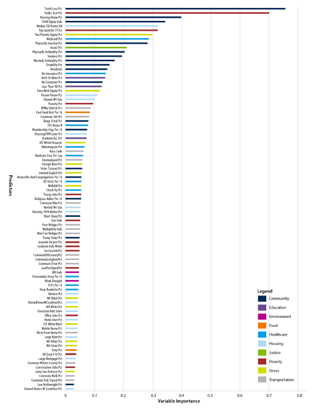
Figure 2 shows the 89 variables retained in the final model and how they ranked in terms of variable importance; Supplement Exhibit 1 provides the complete list of candidate measures. The most important individual predictors—in terms of VI—included percentage with tooth loss; percentage receiving public assistance, including food and heating assistance; percentage of the population in nursing homes; the Child Opportunity Index; and owner-occupied property values.

Figure 2.Variable Importance Rankings in the Pilot Ohio Model

Descriptive Characteristics: Ohio

Table 1 provides comparative statistics for Ohio—overall and in the highest- and lowest-risk deciles of the LSI score. We show both the characteristics of the outcome measure and of the top 10 predictors in terms of variable importance.

The values for many predictors vary starkly between the highest-decile and lowest-decile areas. In the highest-decile neighborhoods, nearly half of residents were receiving public assistance (e.g., the Supplemental Nutrition Assistance Program, or SNAP), compared with only 3 percent of those in the lowest-decile neighborhoods. The percentage of residents receiving public assistance is a poverty measure, but it also reflects state policy: the average SNAP benefit in Ohio in 2015 was $126 per month (Ohio Department of Job and Family Services, 2016). Similarly, property values are more than just a measure of relative affluence—they also reflect the legacy of racism, segregation, and historical redlining (Krieger et al., 2016). In the lowest-decile neighborhoods, property values were nearly 4.5 times higher than in the highest-decile neighborhoods.

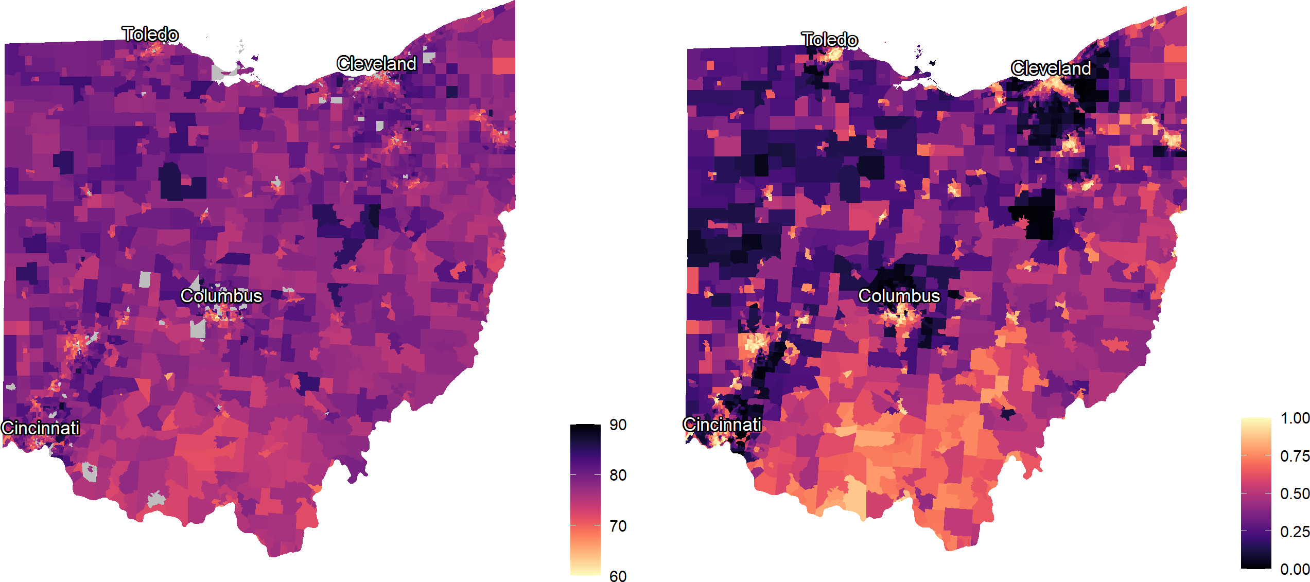
Figure 3 provides maps of the tract-level outcome, LE at birth (on left), and LSI scores (on right) in Ohio. The maps identify, in bright yellow, areas in urban cores and in the southern Appalachian areas of Ohio where community-level social inequities are more prevalent.

Figure 3.Maps of life expectancy (left) and local social inequity (right) by Ohio Census tract (n = 2,949)

Source: Authors’ analysis of life expectancy (LE) and social determinants data in Ohio Census tracts. Brighter yellow indicates shorter LE and higher local social inequity (LSI) scores; dark purple indicates longer LE and lower LSI scores.

Covariate Balance Between the Ohio CPC and Comparison Groups

Table 2 shows the covariate balance between the Ohio CPC and comparison groups for the study sample in the last baseline year for the overall study sample (2016). The analysis estimated propensity scores in each analysis year by using logistic regressions in which the dependent variable was an indicator of inclusion in the Ohio CPC group. Although the analysis calculated propensity scores in each analysis year, means and standardized differences were similar across years, so covariate balance results are presented for the last baseline year only. Before propensity score weighting, standardized differences were greater than 0.10 for some individual- and county-level characteristics. After propensity score weighting, standardized differences were all below the 0.10 threshold, indicating an acceptable level of covariate balance.

Multivariate Modeling Results

Table 3 shows the estimates of the Ohio CPC model on total PBPM, inpatient admissions, ED visits, and readmissions for Medicaid beneficiaries attributed to Ohio CPC practices relative to comparison beneficiaries in a D-in-D model that uses the LSI score as a covariate. The “standard” column in Table 3 also shows D-in-D estimates for the same outcomes from a model that uses county-level covariates from the Area Health Resources Files. A negative value for the regression-adjusted D-in-D corresponds to a greater decrease or a smaller increase in an outcome after the implementation of Ohio CPC relative to the comparison group. A positive value corresponds to a greater increase or a smaller decrease in an outcome in the Ohio CPC group relative to the comparison group after Ohio CPC implementation. The relative difference is the D-in-D estimate as a percentage of the Ohio CPC baseline period adjusted mean.

The following were results from the model that included the LSI score:

1. Total spending per beneficiary per month (PBPM) increased for both Medicaid beneficiaries attributed to the Ohio CPC and the comparison group but increased by $8.37 less ($9.31 less in the standard model) for the Ohio CPC group during the first 2 years of Ohio CPC implementation (P<.001).

2. Inpatient admissions decreased for both Medicaid beneficiaries attributed to Ohio CPC and the comparison group but decreased by 11.99 more admissions per 1,000 beneficiaries (11.85 more admissions per 1,000 beneficiaries in the standard model) for the Ohio CPC group during the first 2 years of Ohio CPC implementation (P < 0.001).

3. ED visits decreased for the Ohio CPC group and increased for comparison beneficiaries, leading to a relative decrease of 24.80 visits per 1,000 beneficiaries (17.79 visits per 1,000 beneficiaries in the standard model) for Medicaid beneficiaries attributed to Ohio CPC practices (P < 0.001).

4. Readmissions within 30 days of discharge increased for both Medicaid beneficiaries attributed to Ohio CPC and the comparison group but increased by 5.14 fewer readmissions per 1,000 discharges (5.63 fewer readmissions per 1,000 discharges in the standard model) for the Ohio CPC group during the first 2 years of Ohio CPC implementation (P = 0.02).

We compared the model that excluded the LSI score but included additional area-level covariates with the model that included the LSI score. The impact estimates remained significant for all outcomes, and including the single LSI score variable in lieu of several area-level covariates resulted in significant differences by LSI in Ohio CPC’s impacts on total spending, inpatient admissions, ED visits, and readmissions. Because a D-in-D model with the LSI score was also more parsimonious than the model with area-level variables and produces more accurate estimates (in terms of narrower Confidence Intervals), there are likely further opportunities to apply the LSI score to impact evaluations.

Discussion

Our LSI score, piloted in Ohio, explains 73 percent of the 29-year variance in LE at birth, with a mean squared error of 4.47. After developing the scores for Ohio, we validated them in several ways, including by evaluating their performance after linking with individual data in the SIM2 evaluation and by benchmarking their performance against alternative, commonly used indices, which explain only 50 to 63 percent of variation in CT-level LE in Ohio. Thus, we find substantial improvement in variance explained relative to other composite measures of SDoH.

It is important to note that the measures against which we compare our performance were not developed to predict or explain LE, whereas ours was. However, we contend that if the comparison composite measures we identified were able to explain variance in LE or other population health outcomes, they could be more useful to the field. As Allik and colleagues wrote in 2020:

Comparisons of indicators and measures have shown that those with a strong foundation in theory are better able to explain variations in health… [A] combined measure should be better able to capture the unmeasured concept of deprivation than the individual indicators themselves. Empirically, this should be reflected in the composite measure having a stronger association to the outcome of interest than any of the variables on their own (Allik et al., 2020).

Several prior studies have used RF models to predict LE. Meshram used RFs to model country-level LE on health outcomes and a few SDoH measures (schooling, GDP), and they compared the RF results with a decision tree model and OLS to find that their RF is the best performing model (Meshram, 2020). Schultz et. al. predicted LE using the individual items of the Frailty Index. They found that RF outperformed OLS and Elastic Net in terms of R² and median error and that using the individual items of the Frailty Index was more accurate than the Frailty Index itself (Schultz et al., 2020). Makridis et al. compared a few ML models to (1) predict the well-being index composite score and (2) classify US military veterans as having high vs. low physical well-being (Makridis et al., 2021). They compared standard methods (OLS and logistic regression) with ML methods (XGBoost and support vector machine) (Makridis et al., 2021). For both model sets, they found XGBoost, a tree-based method (like RF) to perform the best, but their results “suggest that additional measures of socio-economic characteristics are required to better predict physical well-being, particularly among vulnerable groups.” (Makridis et al., 2021)

Limitations

Our findings should be interpreted in light of several limitations and caveats. First, we acknowledge the dangers of ecological fallacy inherent in small-area estimation. Individual-level data are needed to study individual-level outcomes. Thus, while the scores and data are useful on their own as measures of population health, they need to be linked to individual-level data to best make predictions about individuals, as we have demonstrated in the SIM2 evaluation. Similarly, bias may arise if the outcome of interest is from a different era than our outcome measure and predictor data. Changes in area-level characteristics over time are inevitable, and RF models cannot extrapolate a linear trend. We recognize the need to update the model and scores when new LE estimates and predictor data are released. Although it may be possible to generate LSI scores on an annual basis given an annual outcome measure, the current scores are limited to a single point in time and thus are not suitable for measuring progress in reducing health inequities.

One important limitation of this study is that we only estimate a predictive model, without regard to causality. Thus, the variable importance rankings should be interpreted as indicating what is driving the algorithm—not necessarily what is important to policy or practice. Certainly, some of the top predictors could potentially be amenable to interventions, but the goal of this study was not to identify actionable factors for interventions. It was to create an accurate, equity-focused composite measure of SDoH predicting a core population health outcome.

Implications for Policy and Practice

SDoH are typically not accounted for in risk adjustment models, even though, like age, social factors influence health care outcomes and are not a consequence of the quality of healthcare delivery. When social risk factors are not adjusted for in these models, this can result in lower payments to providers who care for patients with higher social risk compared with providers who care for patients with lower social risk, when all else is equal (Ash et al., 2017; National Academies of Sciences, Engineering, and Medicine, 2017). This creates incentives to avoid caring for populations with social risk factors (National Academies of Sciences, Engineering, and Medicine, 2017) which limits the ability of VBP programs to address pervasive health inequities. Several recent publications have noted that most VBP models do not consider health inequities caused by social factors (Ash et al., 2017; Liao, Lavizzo-Mourey, et al., 2021; Sandhu et al., 2020; Werner et al., 2021), with the notable exception of the Medicare ACO REACH Model, which begins in 2023 (Halpern & Holden, 2012). There is some evidence that certain models have actually exacerbated health inequities (Liao, Huang, et al., 2021; Yasaitis et al., 2016). This past year, the CMS Innovation Center made an explicit goal of embedding health equity in all their healthcare models (Menzin et al., 2011). This will require comprehensive tools to measure and account for social risk factors in these payment models.

Including social factors in risk adjustment has been shown to reduce underpayments to providers that serve vulnerable populations (Ash et al., 2017). There are examples of healthcare systems that adjust for social factors, including Massachusetts (Lines et al., 2019), the UK, and New Zealand (Huffstetler & Phillips, 2019). However, social risk adjustment remains controversial. Several recent articles have outlined arguments for and against social risk adjustment in value-based care (Fiscella et al., 2014; Joynt et al., 2017; Nerenz et al., 2021; Phillips et al., 2021; Sheingold et al., 2021; Tran, 2020). These arguments are also reflected in a series of reports from the Department of Health and Human Services (Cubanski et al., 2018; Gold et al., 2007) and the National Academies of Sciences, Engineering, and Medicine (NASEM) (National Academies of Sciences, Engineering, and Medicine, 2017), stemming from the 2014 Improving Medicare Post-Acute Care Transformation (IMPACT) Act, which required an examination of social risk and performance in VBP programs. NASEM has argued that payment adjustments can be made to avoid underpaying providers that serve socially at-risk patients by accounting for the increased resources, or estimated costs, that are required to care for more socially at-risk populations (National Academies of Sciences, Engineering, and Medicine, 2017). These resources can be used to invest in reducing those disparities while improving efficiency and quality of care (National Academies of Sciences, Engineering, and Medicine, 2017). NASEM also recommended that CT-level compositional measures of social risk factors can be used as a good proxy for individual-level data in calculations of these adjustments (National Academies of Sciences, Engineering, and Medicine, 2017). We believe that the LSI is such a measure and that it could be used both in payment adjustments and to identify populations for targeted investment.

The Department of Health and Human Services has acknowledged the need for greater payment support for improving care for patients with social risk, but unlike NASEM, they have not supported social risk adjustment, arguing it would mask disparities (Sheingold et al., 2021). We do not agree that social risk adjustment masks disparities. Adjusting for social factors does not remove the requirement to address those social factors; rather, it directs more funds to addressing those factors. It is also important to note that social risk adjustment is not likely to end health disparities on its own (Damberg et al., 2015), partly because unequal access to care may still result in underprediction of expenditures when social factors are included in risk adjustment models (Damberg et al., 2015; Obermeyer et al., 2019). In addition to social risk adjustment, stratification (Cubanski et al., 2018; National Academies of Sciences, Engineering, and Medicine, 2017) or post-adjustment (Damberg et al., 2015; Phillips et al., 2021) based on social factors can also be used to further ensure appropriate adjustment of payments for social factors.

Disparities in LE are related to numerous social factors (Dimick et al., 2013; Singh et al., 2017). Our approach to creating a composite SDoH index uses modern computing power to provide a new measure that is robust, comprehensive, cross-disciplinary, spatially refined, and highly predictive of a health-equity-centered population health outcome. Considering a broader array of SDoH measures provides a more complete and higher-resolution picture of the relative risks of neighborhoods across Ohio. Accurate multidimensional, cross-sector, small-area social risk scores could be useful in understanding the impact of healthcare innovations, payment models, and interventions on social drivers of health on high-risk communities; identifying neighborhoods and areas at highest risk of poor outcomes for better targeting of interventions and resources; and accounting for factors outside of providers’ control for more fair and equitable performance/quality measurement and reimbursement.

Acknowledgments

Our team has included more than 20 contributors since 2019. The co-authors gratefully acknowledge the input and contributions of the following additional current and former RTI staff (in alphabetical order): Monica Borges, Elena Bravo-Taylor, Anusha Chaudhry, Josh Clemson, Denise Clayton, Erin Erikson, Sara Freeman, Mark Hatem, Ariella Hirsch, Marc Horvath, Yevgeniya Kaganova, Krish Maypole, Marisa Morrison, Rasika Ramanan, Emily Schneider, Clyde Schwab, Kara Sokol, and Joe Wasserman.

Portions of this analysis were previously published in blog form at https://www.themedicalcareblog.com/artificially-intelligent-social-risk-adjustment/ and presented at Health Information and Management Systems Society, August 2021, and the Academy Health National Health Policy Conference and Health Datapalooza, February 2021.

RTI Press Associate Editor: Cynthia Bland